Page 90 - Applied Numerical Methods Using MATLAB

SOLVING A SYSTEM OF LINEAR EQUATIONS 79
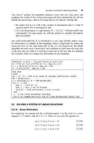
“do_rlse.m” updates the parameter estimates every time new data arrive and
compares the results of the on-line processing with those obtained by the off-line
(batch job) processing—that is, by using Eq.(2.1.12) directly. Noting that

T
ž the matrix [A A k ]aswellas b k consists of information and is a kind of
k
squared matrix that is nonnegative, and
T
T
ž [A A k ] will get larger, or, equivalently, P k = [A A k ] −1 will get smaller and,
k k
consequently, the gain matrix K k will get smaller as valuable information
data accumulate,
one could understand that P k is initialized to a very large identity matrix, since
no information is available in the beginning. Since a large/small P k makes the
correction term on the right-hand side of Eq. (2.1.16) large/small, the RLSE
algorithm becomes more conservative and reluctant to learn from the new data
as the data pile up, while it is willing to make use of the new data for updating
the estimates when it is hungry for information in the beginning.

function [x,K,P] = rlse_online(aT_k1,b_k1,x,P)
K = P*aT_k1’/(aT_k1*P*aT_k1’+1); %Eq.(2.1.17)
x = x +K*(b_k1-aT_k1*x); %Eq.(2.1.16)
P = P-K*aT_k1*P; %Eq.(2.1.18)
%do_rlse
clear
xo = [2 1]’; %The true value of unknown coefficient vector
NA = length(xo);
x = zeros(NA,1); P = 100*eye(NA,NA);
for k = 1:100
A(k,:) = [k*0.01 1];
b(k,:) = A(k,:)*xo +0.2*rand;
[x,K,P] = rlse_online(A(k,:),b(k,:),x,P);
end
x % the final parameter estimate
A\b % for comparison with the off-line processing (batch job)

2.2 SOLVING A SYSTEM OF LINEAR EQUATIONS

2.2.16 Gauss Elimination

For simplicity, we assume that the coefficient matrix A in Eq. (2.0.1) is a non-
singular 3 × 3matrixwith M = N = 3. Then we can write the equation as

(2.2.0a)
a 11 x 1 + a 12 x 2 + a 13 x 3 = b 1
a 21 x 1 + a 22 x 2 + a 23 x 3 = b 2 (2.2.0b)
a 31 x 1 + a 32 x 2 + a 33 x 3 = b 3 (2.2.0c)