Page 88 - Applied Numerical Methods Using MATLAB

SOLUTION FOR A SYSTEM OF LINEAR EQUATIONS 77
the resistance R[ ] of a resistor as

c 1 t + c 2 = R

and we have lots of experimental data {(t 1 ,R 1 ), (t 2 ,R 2 ), .. .,(t k ,R k )} collected
up to time k. Since the above equation cannot be satisfied for all the data with any
value of the parameters c 1 and c 2 , we should try to get the parameter estimates
that are optimal in some sense. This corresponds to the overdetermined case dealt
with in the previous section and can be formulated as an LSE problem that we
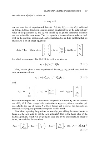
must solve a set of linear equations

   
t 1 1 R 1
 
t
1


A k x k ≈ b k , where A k =  2  , x k = c 1,k , and b k =  R 2 
 ·  · 
·  c 2,k
t k 1 R k
for which we can apply Eq. (2.1.10) to get the solution as
T −1 T
x k = [A A k ] A b k (2.1.11)
k
k
Now, we are given a new experimental data (t k+1 , R k+1 ) and must find the
new parameter estimate
−1
x k+1 = [A T A k+1 ] A T b (2.1.12)
k+1 k+1 k+1
with
   
1
t 1 R 1

 · ·  c 1,k+1  · 
A k+1 =   , x k+1 = , and b k+1 =  
 t k c 2,k+1  R k 
1 
t k+1 1 R k+1
How do we compute this? If we discard the previous estimate x k and make direct
use of Eq. (2.1.12) to compute the next estimate x k+1 every time a new data pair
is available, the size of matrix A will get bigger and bigger as the data pile up,
eventually defying any powerful computer in this world.
How about updating the previous estimate by just adding the correction term
based on the new data to get the new estimate? This is the basic idea of the
RLSE algorithm, which we are going to trace and try to understand. In order to
do so, let us define the notations

A k t k+1 b k T −1
A k+1 = T , a k+1 = , b k+1 = , and P k = [A A k ]
k
a 1 R k+1
k+1
(2.1.13)