Page 92 - Applied Numerical Methods Using MATLAB

SOLVING A SYSTEM OF LINEAR EQUATIONS 81
We call this procedure ‘backward substitution’ and can generalize the solution
formula (2.2.6) as

M

(m−1) (m−1)
(m−1)
x m = b − a x n /a for m = M, M − 1,... , 1
m mn mm
n=m+1
(2.2.7)
In this way, the Gauss elimination procedure consists of two steps, namely,
forward elimination and backward substitution. Noting that
ž this procedure has nothing to do with the specific values of the unknown
variable x m ’s and involves only the coefficients, and
ž the formulas (2.2.5a) on the coefficient matrix A and (2.2.5b) on the RHS
(right-hand side) vector b conform with each other,

we will augment A with b and put the formulas (2.2.5a,b) together into one
framework when programming the Gauss forward elimination procedure.

2.2.2 Partial Pivoting
(k−1)
The core formula (2.2.5) used for Gauss elimination requires division by a kk
(k−1)
at the kth stage, where a kk is the diagonal element in the kth row. What if
(k−1)
a = 0? In such a case, it is customary to switch the kth row and another row
kk
below it having the element of the largest absolute value in the kth column. This
procedure, called ‘partial pivoting’, is recommended for reducing the round-off
(k−1)
error even in the case where the kth pivot a is not zero.
kk
Let us consider the following example:
     
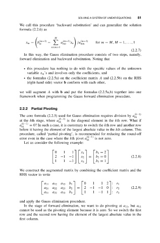
0 1 1 x 1 b 1 = 2
 2 −1 −1   x 2  =  b 2 = 0  (2.2.8)
1 1 −1 x 3 b 3 = 1

We construct the augmented matrix by combining the coefficient matrix and the
RHS vector to write

   
0 1
a 11 a 12 a 13 b 1 1 2 : r 1
a 21 a 22 a 23 b 2 2 −1 −10 : r 2
  =   (2.2.9)
1
a 31 a 32 a 33 b 3 1 −11 : r 3
and apply the Gauss elimination procedure.
In the stage of forward elimination, we want to do pivoting at a 11 , but a 11
cannot be used as the pivoting element because it is zero. So we switch the first
row and the second row having the element of the largest absolute value in the
first column.