Page 93 - Applied Numerical Methods Using MATLAB

82 SYSTEM OF LINEAR EQUATIONS
 (1) (1) (1) (1)    (1)
a a a b 2 −1 −10 : r
11 12 13 1 1
 (1) (1) (1)    (1)

 a a a b (1)  =  0 1 1 2 : r (2.2.10a)
 21 22 23 2    2
(1) (1) (1) (1) (1)
a a a b 1 1 −11 : r
31 32 33 3 3
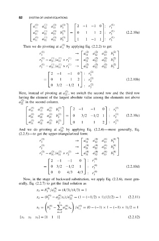
Then we do pivoting at a (1) by applying Eq. (2.2.2) to get
11
(1)  (2) (2) (2) (2) 
r → a a a b
1 11 12 13 1
(1) (1) (1) (1)  (2) (2) (2) 
r − a /a × r →  a a a b (2) 
2 21 11 1  21 22 23 2 
(1) (1) (1) (1) (2) (2) (2) (2)
r − a /a × r → a a a b
3 31 11 1 31 32 33 3
(2)
2 −1 −1 0 : r
 
1
=  0 1 1 2  : r (2) (2.2.10b)


2
03/2 −1/21 : r (2)
3
(2)
Here, instead of pivoting at a , we switch the second row and the third row
22
having the element of the largest absolute value among the elements not above
(2)
a in the second column.
22
 (3) (3) (3) (3)    (3)
a a a b 2 −1 −1 0 : r
11 12 13 1 1
 (3) (3) (3)    (3)
a a a b r
 (3)  =  0 3/2 −1/21  : (2.2.10c)
 21 22 23 2    2
(3) (3) (3) (3) (3)
a a a b 0 1 1 2 : r
31 32 33 3 3
(3)
Andwedopivoting at a by applying Eq. (2.2.4)—more generally, Eq.
22
(2.2.5)—to get the upper-triangularized form:
(3)  (4) (4) (4) (4) 
r → a a a b
1 11 12 13 1
(3)  (4) (4) (4) 
r →  a a a b (4) 
2  21 22 23 2 
(3) (3) (3) (3) (4) (4) (4) (4)
r − a /a × r → a a a b
3 31 11 2 31 32 33 3
2 −1 −1 0 : r 1
  (4)
=  03/2 −1/2 1  : r (4) (2.2.10d)


2
0 0 4/3 4/3 : r (4)
3
Now, in the stage of backward substitution, we apply Eq. (2.2.6), more gen-
erally, Eq. (2.2.7) to get the final solution as
(4) (4)
x 3 = b /a = (4/3)/(4/3) = 1
3 33
(4)
x 2 = (b (4) − a x 3 )/a (4) = (1 − (−1/2) × 1)/(3/2) = 1 (2.2.11)
2 23 22
3

(4) (4) (4)
x 1 = b − a x n /a = (0 − (−1) × 1 − (−1) × 1)/2 = 1
1 1n 11
n=2
[x 1 x 2 x 3 ] = [1 1 1] (2.2.12)