Page 89 - Applied Numerical Methods Using MATLAB

78 SYSTEM OF LINEAR EQUATIONS
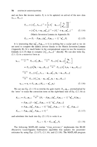
and see how the inverse matrix P k is to be updated on arrival of the new data
(t k+1 , R k+1 ).
−1

T −1 T A k
P k+1 = [A k+1 A k+1 ] = [ A k a k+1 ] T
a
k+1
T
= [A A k + a k+1 a T ] −1 = [P −1 + a k+1 a T ] −1 (2.1.14)
k k+1 k k+1
(Matrix Inversion Lemma in Appendix B)
−1 T
P
P
P k+1 = P k − P k a k+1 [a T k+1 k a k+1 + 1] a k+1 k (2.1.15)
P
It is interesting that [a T k+1 k a k+1 + 1] is nothing but a scalar and so we do
not need to compute the matrix inverse thanks to the Matrix Inversion Lemma
(Appendix B). It is much better in the computational aspect to use the recursive
formula (2.1.15) than to compute [A T A k+1 ] −1 directly. We can also write Eq.
k+1
(2.1.12) in a recursive form as

(2.1.12, 14) T (2.1.13) T b k
b
x k+1 = P k+1 A k+1 k+1 = P k+1 [A a k+1 ]
k
R k+1
T
T
= P k+1 [A b k + a k+1 R k+1 ] (2.1.11) P k+1 [A A k x k + a k+1 R k+1 ]
=
k k
(2.1.13) T T
= P k+1 [(A A k+1 − a k+1 a )x k + a k+1 R k+1 ]
k+1 k+1
(2.1.13) −1 T
x
x
= P k+1 [P k+1 k − a k+1 a k+1 k + a k+1 R k+1 ]
x k+1 = x k + P k+1 a k+1 (R k+1 − a T k+1 k ) (2.1.16)
x
We can use Eq. (2.1.15) to rewrite the gain matrix P k+1 a k+1 premultiplied by
the ‘error’ to make the correction term on the right-hand side of Eq. (2.1.16) as
(2.1.15) T −1 T
P
P
K k+1 = P k+1 a k+1 = [P k − P k a k+1 [a k+1 k a k+1 + 1] a k+1 k ]a k+1
−1 T
P
P
= P k a k+1 [I − [a T k+1 k a k+1 + 1] a k+1 k a k+1 ]
−1
P
P
= P k a k+1 [a T k+1 k a k+1 + 1] {[a T k+1 k a k+1 + 1] − a T k+1 k a k+1 }
P
K k+1 = P k a k+1 [a T k+1 k a k+1 + 1] −1 (2.1.17)
P
and substitute this back into Eq. (2.1.15) to write it as
P k+1 = P k − K k+1 a T k+1 k (2.1.18)
P
The following MATLAB routine “rlse_online()” implements this RLSE
(Recursive Least-Squares Estimation) algorithm that updates the parameter
estimates by using Eqs. (2.1.17), (2.1.16), and (2.1.18). The MATLAB program