Page 84 - Applied Numerical Methods Using MATLAB

SOLUTION FOR A SYSTEM OF LINEAR EQUATIONS 73
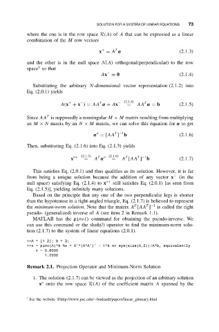
where the one is in the row space R(A) of A that can be expressed as a linear
combination of the M row vectors
T
x = A α (2.1.3)
+
and the other is in the null space N(A) orthogonal(perpendicular) to the row
1
space so that
Ax = 0 (2.1.4)
−
Substituting the arbitrary N-dimensional vector representation (2.1.2) into
Eq. (2.0.1) yields

T
T
−
A(x + x ) = AA α + Ax − (2.1.4) AA α = b (2.1.5)
+
=
T
Since AA is supposedly a nonsingular M × M matrix resulting from multiplying
an M × N matrix by an N × M matrix, we can solve this equation for α to get
T −1
o
α = [AA ] b (2.1.6)
Then, substituting Eq. (2.1.6) into Eq. (2.1.3) yields
o+ (2.1.3) T o (2.1.6) T T −1
x = A α = A [AA ] b (2.1.7)
This satisfies Eq. (2.0.1) and thus qualifies as its solution. However, it is far
from being a unique solution because the addition of any vector x − (in the
null space) satisfying Eq. (2.1.4) to x o+ still satisfies Eq. (2.0.1) [as seen from
Eq. (2.1.5)], yielding infinitely many solutions.
Based on the principle that any one of the two perpendicular legs is shorter
than the hypotenuse in a right-angled triangle, Eq. (2.1.7) is believed to represent
T −1
T
the minimum-norm solution. Note that the matrix A [AA ] is called the right
pseudo- (generalized) inverse of A (see item 2 in Remark 1.1).
MATLAB has the pinv() command for obtaining the pseudo-inverse. We
can use this command or the slash(/) operator to find the minimum-norm solu-
tion (2.1.7) to the system of linear equations (2.0.1).

>>A=[12];b=3;
>>x = pinv(A)*b %x = A’*(A*A’)^ - 1*b or eye(size(A,2))/A*b, equivalently
x = 0.6000
1.2000
Remark 2.1. Projection Operator and Minimum-Norm Solution

1. The solution (2.1.7) can be viewed as the projection of an arbitrary solution
o
x onto the row space R(A) of the coefficient matrix A spanned by the

1 See the website @http://www.psc.edu/∼burkardt/papers/linear glossary.html