Page 99 - Applied Numerical Methods Using MATLAB

88 SYSTEM OF LINEAR EQUATIONS
factor, we cannot say that some pivoting scheme always yields better solution than
other pivoting schemes, because the result depends on the random round-off error as
well as the pivoting scheme (see Problem 2.2). But, in most cases, the scaled partial
pivoting shows a reasonably good performance and that is why we adopt it in our
routine “gauss()”.
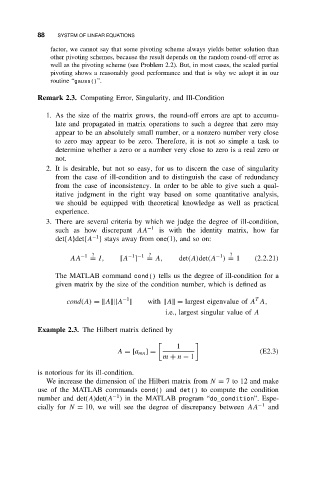
Remark 2.3. Computing Error, Singularity, and Ill-Condition

1. As the size of the matrix grows, the round-off errors are apt to accumu-
late and propagated in matrix operations to such a degree that zero may
appear to be an absolutely small number, or a nonzero number very close
to zero may appear to be zero. Therefore, it is not so simple a task to
determine whether a zero or a number very close to zero is a real zero or
not.
2. It is desirable, but not so easy, for us to discern the case of singularity
from the case of ill-condition and to distinguish the case of redundancy
from the case of inconsistency. In order to be able to give such a qual-
itative judgment in the right way based on some quantitative analysis,
we should be equipped with theoretical knowledge as well as practical
experience.
3. There are several criteria by which we judge the degree of ill-condition,
such as how discrepant AA −1 is with the identity matrix, how far
−1
det{A}det{A } stays away from one(1), and so on:
?
−1 −1 ?
−1
= I,
AA −1 ? [A ] = A, det(A)det(A ) = 1 (2.2.21)
The MATLAB command cond() tells us the degree of ill-condition for a
given matrix by the size of the condition number, which is defined as
−1 T
cond(A) =||A||||A || with ||A|| = largest eigenvalue of A A,
i.e., largest singular value of A

Example 2.3. The Hilbert matrix defined by

1
A = [a mn ] = (E2.3)
m + n − 1
is notorious for its ill-condition.
We increase the dimension of the Hilbert matrix from N = 7to 12and make
use of the MATLAB commands cond() and det() to compute the condition
−1
number and det(A)det(A ) in the MATLAB program “do_condition”. Espe-
cially for N = 10, we will see the degree of discrepancy between AA −1 and