Page 100 - Applied Numerical Methods Using MATLAB

SOLVING A SYSTEM OF LINEAR EQUATIONS 89
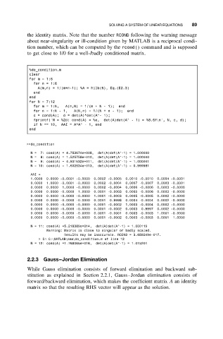
the identity matrix. Note that the number RCOND following the warning message
about near-singularity or ill-condition given by MATLAB is a reciprocal condi-
tion number, which can be computed by the rcond() command and is supposed
to get close to 1/0 for a well-/badly conditioned matrix.

%do_condition.m
clear
for m = 1:6
for n = 1:6
A(m,n) = 1/(m+n-1); %A = hilb(6), Eq.(E2.3)
end
end
for N = 7:12
for m = 1:N, A(m,N) = 1/(m+N-1); end
for n = 1:N - 1, A(N,n) = 1/(N+n-1); end
c = cond(A); d = det(A)*det(A^- 1);
fprintf(’N = %2d: cond(A) = %e, det(A)det(A^ - 1) = %8.6f\n’, N, c, d);
if N == 10, AAI = A*A^ - 1, end
end

>>do_condition
N = 7: cond(A) = 4.753674e+008, det(A)det(A^-1) = 1.000000
N = 8: cond(A) = 1.525758e+010, det(A)det(A^-1) = 1.000000
N = 9: cond(A) = 4.931532e+011, det(A)det(A^-1) = 1.000001
N = 10: cond(A) = 1.602534e+013, det(A)det(A^-1) = 0.999981
AAI =
1.0000 0.0000 -0.0001 -0.0000 0.0002 -0.0005 0.0010 -0.0010 0.0004 -0.0001
0.0000 1.0000 -0.0001 -0.0000 0.0002 -0.0004 0.0007 -0.0007 0.0003 -0.0001
0.0000 0.0000 1.0000 -0.0000 0.0002 -0.0004 0.0006 -0.0006 0.0003 -0.0000
0.0000 0.0000 -0.0000 1.0000 0.0001 -0.0003 0.0005 -0.0006 0.0003 -0.0000
0.0000 0.0000 -0.0000 -0.0000 1.0001 -0.0003 0.0005 -0.0005 0.0002 -0.0000
0.0000 0.0000 -0.0000 -0.0000 0.0001 0.9998 0.0004 -0.0004 0.0002 -0.0000
0.0000 0.0000 -0.0000 -0.0000 0.0001 -0.0002 1.0003 -0.0004 0.0002 -0.0000
0.0000 0.0000 -0.0000 -0.0000 0.0001 -0.0002 0.0003 0.9997 0.0002 -0.0000
0.0000 0.0000 -0.0000 -0.0000 0.0001 -0.0001 0.0003 -0.0003 1.0001 -0.0000
0.0000 0.0000 -0.0000 -0.0000 0.0001 -0.0002 0.0003 -0.0003 0.0001 1.0000
N = 11: cond(A) =5.218389e+014, det(A)det(A^-1) = 1.000119
Warning: Matrix is close to singular or badly scaled.
Results may be inaccurate. RCOND = 3.659249e-017.
>InC:\MATLAB\nma\do_condition.m at line 12
N = 12: cond(A) =1.768065e+016, det(A)det(A^-1) = 1.015201

2.2.3 Gauss–Jordan Elimination

While Gauss elimination consists of forward elimination and backward sub-
stitution as explained in Section 2.2.1, Gauss–Jordan elimination consists of
forward/backward elimination, which makes the coefficient matrix A an identity
matrix so that the resulting RHS vector will appear as the solution.