Page 102 - Applied Numerical Methods Using MATLAB
P. 102

SOLVING A SYSTEM OF LINEAR EQUATIONS  91
            which denotes a system of linear equations having an identity matrix as the
            coefficient matrix
                                       []    [3]  [2]  [1] T
                                I x = b = [ b    b   b   ]
                                             1    2   3
                                               []
            and, consequently, take the RHS vector b as the final solution.
              Note that we don’t have to distinguish the two steps, the forward/backward
            elimination. In other words, during the forward elimination, we do the pivot-
            ing operations in such a way that the pivot becomes one and other elements
            above/below the pivot in the same column become zeros.
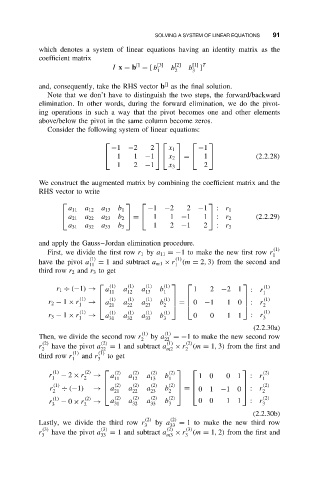
              Consider the following system of linear equations:

                                                      
                                −1 −2      2    x 1     −1
                               1     1  −1   x 2    =   1         (2.2.28)
                                 1    2  −1     x 3       2

            We construct the augmented matrix by combining the coefficient matrix and the
            RHS vector to write
                                                        
                    a 11  a 12  a 13  b 1  −1 −2     2  −1   : r 1
                   a 21  a 22  a 23  b 2    =   1  1 −1  1  : r 2   (2.2.29)
                    a 31  a 32  a 33  b 3   1   2 −1      2  : r 3

            and apply the Gauss–Jordan elimination procedure.
                                                                             (1)
              First, we divide the first row r 1 by a 11 =−1 to make the new first row r
                                                                             1
                          (1)                     (1)
            have the pivot a  = 1 and subtract a m1 × r  (m = 2, 3) from the second and
                          11                      1
            third row r 2 and r 3 to get
                              (1)  (1)  (1)  (1)                      (1)
                 r 1 ÷ (−1) →  a   a    a    b         1   2  −21      : r
                               11   12   13   1                           1
                       (1)    (1)  (1)  (1)                           (1)
              r 2 − 1 × r  →   a  a    a    b  (1)   =    0  −1  1  0    : r
                       1     21    22   23   2                        2
                       (1)     (1)  (1)  (1)  (1)                         (1)
              r 3 − 1 × r  →  a    a    a    b         0   0    1  1   : r
                       1       31   32   33   3                           3
                                                                       (2.2.30a)
                                        (1)    (1)
            Then, we divide the second row r  by a  =−1 to make the new second row
                                        2      22
             (2)             (2)               (1)   (2)
            r  have the pivot a  = 1 and subtract a  × r (m = 1, 3) from the first and
             2               22                m2   2
                     (1)    (1)
            third row r  and r  to get
                     1      3
               r  (1)  − 2 × r (2)  →   a (2)  a (2)  a (2)  b (2)        : r  (2)
               1        2        11   12   13   1       10      0  1      1
                (1)             (2)  (2)  (2)                         (2)
               r  ÷ (−1)   →   a    a    a    b  (2)   =    01 −1  0    : r
                2              21    22   23   2                      2
                (1)     (2)      (2)  (2)  (2)  (2)                       (2)
               r  − 0 × r  →    a    a    a    b        00      1  1  : r
               3        2        31   32   33   3                         3
                                                                       (2.2.30b)
                                         (2)    (2)
            Lastly, we divide the third row r  by a  = 1 to make the new third row
                                         3      33
             (3)             (3)               (2)   (3)
            r  have the pivot a  = 1 and subtract a  × r (m = 1, 2) from the first and
             3               33                m3   3
   97   98   99   100   101   102   103   104   105   106   107