Page 107 - Applied Numerical Methods Using MATLAB

96 SYSTEM OF LINEAR EQUATIONS
than to apply the Gauss elimination method. The procedure is as follows:

T
P LU x = b, LU x = P b, U x = L −1 P b, x = U −1 L −1 P b
(2.4.11)
Note that the premultiplication of L −1 and U −1 by a vector can be per-
formed by the forward and backward substitution, respectively. The following
program “do_lu_dcmp.m” applies the LU decomposition method, the Gauss
elimination algorithm, and the MATLAB operators ‘\’and ‘inv’or‘^-1’to
solve Eq. (2.4.10), where A is the five-dimensional Hilbert matrix (introduced
T
o
o
in Example 2.3) and b = Ax with x = [ 111 11 ] . The residual error
||Ax i − b|| of the solutions obtained by the four methods and the numbers of
floating-point operations required for carrying out them are listed in Table 2.1.
The table shows that, once the inverse matrix A −1 is available, the inverse matrix
2
method requiring only N multiplications/additions (N is the dimension of the
coefficient matrix or the number of unknown variables) is the most efficient in
computation, but the worst in accuracy. Therefore, if we need to continually
solve the system of linear equations with the same coefficient matrix A for dif-
ferent RHS vectors, it is a reasonable choice in terms of computation time and
accuracy to save the LU decomposition of the coefficient matrix A and apply the
forward/backward substitution process.

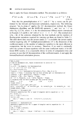
%do_lu_dcmp
% Use LU decomposition, Gauss elimination to solve Ax = b
A = hilb(5);
[L,U,P] = lu_dcmp(A); %LU decomposition
x = [1 -2 3 -4 5 -6 7 -8 9 -10]’;
b = A*x(1:size(A,1));
flops(0), x_lu = backsubst(U,forsubst(L,P*b)); %Eq.(2.4.11)
flps(1) = flops; % assuming that we have already got L\U decomposition
flops(0), x_gs = gauss(A,b); flps(3) = flops;
flops(0), x_bs = A\b; flps(4) = flops;
AI = A^-1; flops(0), x_iv = AI*b; flps(5) = flops;
% assuming that we have already got the inverse matrix
disp(’ x_lu x_gs x_bs x_iv’)
format short e
solutions = [x_lu x_gs x_bs x_iv]
errs = [norm(A*x_lu - b) norm(A*x_gs - b) norm(A*x_bs - b) norm(A*x_iv - b)]
format short, flps
function x = forsubst(L,B)
%forward substitution for a lower-triangular matrix equation Lx = B
N = size(L,1);
x(1,:) = B(1,:)/L(1,1);
for m = 2:N
x(m,:) = (B(m,:)-L(m,1:m - 1)*x(1:m-1,:))/L(m,m);
end
function x = backsubst(U,B)
%backward substitution for a upper-triangular matrix equation Ux = B
N = size(U,2);
x(N,:) = B(N,:)/U(N,N);
for m = N-1: -1:1
x(m,:) = (B(m,:) - U(m,m + 1:N)*x(m + 1:N,:))/U(m,m);
end