Page 112 - Applied Numerical Methods Using MATLAB

ITERATIVE METHODS TO SOLVE EQUATIONS 101
multiprocessor computer capable of parallel processing, each one of N variables
is updated sequentially one by one. Therefore, it is no wonder that we could
speed up the convergence by using all the most recent values of variables for
updating each variable even in the same iteration as follows:
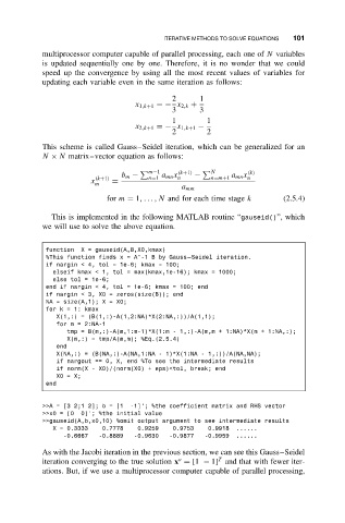
2 1
x 1,k+1 =− x 2,k +
3 3
1 1
x 2,k+1 =− x 1,k+1 −
2 2
This scheme is called Gauss–Seidel iteration, which can be generalized for an
N × N matrix–vector equation as follows:

m−1 (k+1) N (k)
b m − a mn x − a mn x
(k+1) n=1 n n=m+1 n
x =
m
a mm
for m = 1,. ..,N and for each time stage k (2.5.4)
This is implemented in the following MATLAB routine “gauseid()”, which
we will use to solve the above equation.

function X = gauseid(A,B,X0,kmax)
%This function finds x = A^-1 B by Gauss–Seidel iteration.
if nargin < 4, tol = 1e-6; kmax = 100;
elseif kmax < 1, tol = max(kmax,1e-16); kmax = 1000;
else tol = 1e-6;
end if nargin < 4, tol = 1e-6; kmax = 100; end
if nargin < 3, X0 = zeros(size(B)); end
NA = size(A,1);X=X0;
fork=1: kmax
X(1,:) = (B(1,:)-A(1,2:NA)*X(2:NA,:))/A(1,1);
for m = 2:NA-1
tmp = B(m,:)-A(m,1:m-1)*X(1:m - 1,:)-A(m,m + 1:NA)*X(m + 1:NA,:);
X(m,:) = tmp/A(m,m); %Eq.(2.5.4)
end
X(NA,:) = (B(NA,:)-A(NA,1:NA - 1)*X(1:NA - 1,:))/A(NA,NA);
if nargout == 0, X, end %To see the intermediate results
if norm(X - X0)/(norm(X0) + eps)<tol, break; end
X0=X;
end

>>A=[32;1 2];b=[1 -1]’; %the coefficient matrix and RHS vector
>>x0 = [0 0]’; %the initial value
>>gauseid(A,b,x0,10) %omit output argument to see intermediate results
X = 0.3333 0.7778 0.9259 0.9753 0.9918 ......
-0.6667 -0.8889 -0.9630 -0.9877 -0.9959 ......

As with the Jacobi iteration in the previous section, we can see this Gauss–Seidel
o
T
iteration converging to the true solution x = [1 − 1] and that with fewer iter-
ations. But, if we use a multiprocessor computer capable of parallel processing,