Page 115 - Applied Numerical Methods Using MATLAB

104 SYSTEM OF LINEAR EQUATIONS
as illustrated in Section 2.5.1. Then, what is the convergence condition? It is the
diagonal dominancy of coefficient matrix A, which is stated as follows:
N

|a mm | > |a mn | for m = 1, 2,. ..,N (2.5.5)
n =m
This implies that the convergence of the iterative schemes is ensured if, in
each row of coefficient matrix A, the absolute value of the diagonal element
is greater than the sum of the absolute values of the other elements. It should
be noted, however, that this is a sufficient, not a necessary, condition. In other
words, the iterative scheme may work even if the above condition is not strictly
satisfied.
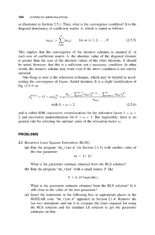
One thing to note is the relaxation technique, which may be helpful in accel-
erating the convergence of Gauss–Seidel iteration. It is a slight modification of
Eq. (2.5.4) as

m−1 (k+1) N (k)
b m − n=1 a mn x n − n=m+1 a mn x n
(k+1)
(k)
x = (1 − ω)x + ω
m m
a mm
with 0 <ω < 2 (2.5.6)
and is called SOR (successive overrelaxation) for the relaxation factor 1 <ω <
2 and successive underrelaxation for 0 <ω < 1. But regrettably, there is no
general rule for selecting the optimal value of the relaxation factor ω.

PROBLEMS

2.1 Recursive Least-Squares Estimation (RLSE)
(a) Run the program ‘do_rlse.m’ (in Section 2.1.4) with another value of
the true parameter
xo=[12]’

What is the parameter estimate obtained from the RLS solution?
(b) Run the program “do_rlse” with a small matrix P like

P = 0.01*eye(NA);

What is the parameter estimate obtained from the RLS solution? Is it
still close to the value of the true parameter?
(c) Insert the statements in the following box at appropriate places in the
MATLAB code “do_rlse.m” appeared in Section 2.1.4. Remove the
last two statements and run it to compare the times required for using
the RLS solution and the standard LS solution to get the parameter
estimates on-line.