Page 119 - Applied Numerical Methods Using MATLAB

108 SYSTEM OF LINEAR EQUATIONS
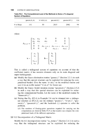
Table P2.4 The Computational Load of the Methods to Solve a Tri-diagonal
System of Equations

gauss(A,b) trid(A,b) gauseid() gauseid1() A\b
# of flops 141 50 2615 2082 94

where

 0 0 0 
a 11 a 12
0 0
 a 21 a 22 a 23 
A N×N =  0 · · · · ·· ·· · 0  ,


0 0 a N−1,N−2 a N−1,N−1 a N−1,N
 
0 0 0 a N,N−1 a NN
   
x 1 b 1
 x 2   b 2 
.  , .
   
x =  b =  
   
x N−1 b N−1
x N b N
This is called a tridiagonal system of equations on account of that the
coefficient matrix A has nonzero elements only on its main diagonal and
super-/subdiagonals.
(a) Modify the Gauss elimination routine “gauss()” (Section 2.2.1) in such
a way that this special structure can be exploited for reducing the com-
putational burden. Give the name ‘trid()’ to the modified routine and
save it in an m-file named “trid.m” for future use.
(b) Modify the Gauss–Seidel iteration routine “gauseid()” (Section 2.5.2)
in such a way that this special structure can be exploited for reduc-
ing the computational burden. Let the name of the modified routine be
“Gauseid1()”.
(c) Noting that Eq. (E2.4) in Example 2.4 can be trimmed into a tridiago-
nal structure as (P2.4.2), use the routines “gauss()”, “trid()”, “gau-
seid()”, “gauseid1()”, and the backslash (\) operator to solve the
problem.
(cf) The numbers of floating-point operations required for carrying out the
computations are listed in Table P2.4 so that readers can compare the com-
putational loads of the different approaches.

2.5 LU Decomposition of a Tridiagonal Matrix
Modify the LU decomposition routine “lu_dcmp()”(Section2.4.1)insucha
way that the tridiagonal structure can be exploited for reducing the