Page 125 - Applied Numerical Methods Using MATLAB

114 SYSTEM OF LINEAR EQUATIONS
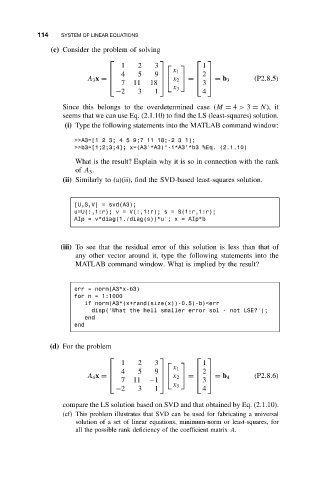
(c) Consider the problem of solving

   
1 2 3   1
x 1
2
 4 5 9   
A 3 x =    x 2  =   = b 3 (P2.8.5)
 7 11 18   3 
x 3
−2 3 1 4
Since this belongs to the overdetermined case (M = 4 > 3 = N), it
seems that we can use Eq. (2.1.10) to find the LS (least-squares) solution.
(i) Type the following statements into the MATLAB command window:
>>A3=[1 2 3; 4 5 9;7 11 18;-2 3 1];
>>b3=[1;2;3;4]; x=(A3’*A3)^-1*A3’*b3 %Eq. (2.1.10)

What is the result? Explain why it is so in connection with the rank
of A 3 .
(ii) Similarly to (a)(ii), find the SVD-based least-squares solution.

[U,S,V] = svd(A3);
u=U(:,1:r); v = V(:,1:r); s = S(1:r,1:r);
AIp = v*diag(1./diag(s))*u’; x = AIp*b

(iii) To see that the residual error of this solution is less than that of
any other vector around it, type the following statements into the
MATLAB command window. What is implied by the result?

err = norm(A3*x-b3)
for n = 1:1000
if norm(A3*(x+rand(size(x))-0.5)-b)<err
disp(’What the hell smaller error sol - not LSE?’);
end
end

(d) For the problem
   
1 2 3   1
x 1
4 5 9 2
   
A 4 x =    x 2  =   = b 4 (P2.8.6)
 7 11 −1   3 
x 3
−2 3 1 4
compare the LS solution based on SVD and that obtained by Eq. (2.1.10).
(cf) This problem illustrates that SVD can be used for fabricating a universal
solution of a set of linear equations, minimum-norm or least-squares, for
all the possible rank deficiency of the coefficient matrix A.