Page 129 - Applied Numerical Methods Using MATLAB

118 INTERPOLATION AND CURVE FITTING
But, as the number of data points increases, so does the number of unknown
variables and equations, consequently, it may be not so easy to solve. That is
why we look for alternatives to get the coefficients {a 0 ,a 1 ,...,a N }.
One of the alternatives is to make use of the Lagrange polynomials

(x − x 1 )(x − x 2 ) ··· (x − x N ) (x − x 0 )(x − x 2 ) ·· · (x − x N )
l N (x)=y 0 + y 1
(x 0 − x 1 )(x 0 − x 2 ) ·· · (x 0 − x N ) (x 1 − x 0 )(x 1 − x 2 ) ··· (x 1 − x N )
(x − x 0 )(x − x 1 ) ·· · (x − x N−1 )
+ ··· + y N
(x N − x 0 )(x N − x 1 ) ·· · (x N − x N−1 )
N N N
k =m x − x k
(x − x k )
l N (x)= = (3.1.3)
N
y m L N,m (x) with L N,m (x)=
m=0 k =m (x m − x k ) k =m x m − x k
It can easily be shown that the graph of this function matches every data point
l N (x m ) = y m ∀ m = 0, 1,...,N (3.1.4)
since the Lagrange coefficient polynomial L N,m (x) is 1 only for x = x m and zero
for all other data points x = x k (k = m). Note that the Nth-degree polynomial
function matching the given N + 1 points is unique and so Eq. (3.1.1) having
the coefficients obtained from Eq. (3.1.2) must be the same as the Lagrange
polynomial (3.1.3).
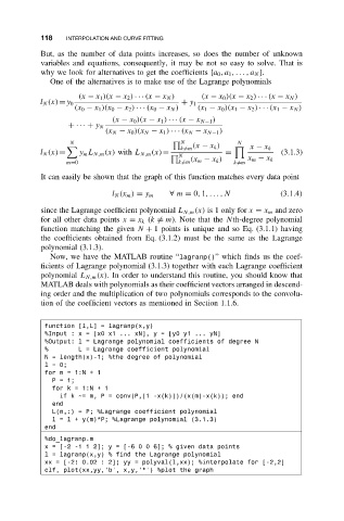
Now, we have the MATLAB routine “lagranp()” which finds us the coef-
ficients of Lagrange polynomial (3.1.3) together with each Lagrange coefficient
polynomial L N,m (x). In order to understand this routine, you should know that
MATLAB deals with polynomials as their coefficient vectors arranged in descend-
ing order and the multiplication of two polynomials corresponds to the convolu-
tion of the coefficient vectors as mentioned in Section 1.1.6.

function [l,L] = lagranp(x,y)
%Input:x=[x0 x1 ... xN], y = [y0 y1 ... yN]
%Output: l = Lagrange polynomial coefficients of degree N
% L = Lagrange coefficient polynomial
N = length(x)-1; %the degree of polynomial
l=0;
for m = 1:N + 1
P=1;
for k = 1:N + 1
if k ~= m, P = conv(P,[1 -x(k)])/(x(m)-x(k)); end
end
L(m,:) = P; %Lagrange coefficient polynomial
l=l+ y(m)*P; %Lagrange polynomial (3.1.3)
end
%do_lagranp.m
x = [-2 -1 1 2]; y = [-6 0 0 6]; % given data points
l = lagranp(x,y) % find the Lagrange polynomial
xx = [-2: 0.02 : 2]; yy = polyval(l,xx); %interpolate for [-2,2]
clf, plot(xx,yy,’b’, x,y,’*’) %plot the graph