Page 131 - Applied Numerical Methods Using MATLAB

120 INTERPOLATION AND CURVE FITTING
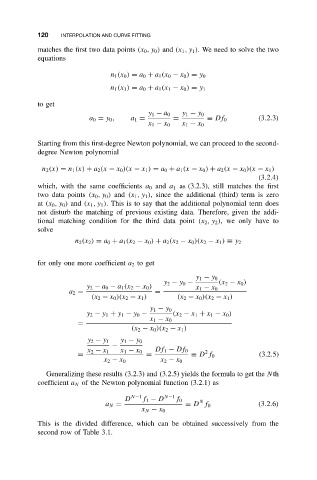
matches the first two data points (x 0 ,y 0 ) and (x 1 ,y 1 ). We need to solve the two
equations

n 1 (x 0 ) = a 0 + a 1 (x 0 − x 0 ) = y 0
n 1 (x 1 ) = a 0 + a 1 (x 1 − x 0 ) = y 1

to get
y 1 − a 0 y 1 − y 0
a 0 = y 0 , a 1 = = ≡ Df 0 (3.2.3)
x 1 − x 0 x 1 − x 0
Starting from this first-degree Newton polynomial, we can proceed to the second-
degree Newton polynomial

n 2 (x) = n 1 (x) + a 2 (x − x 0 )(x − x 1 ) = a 0 + a 1 (x − x 0 ) + a 2 (x − x 0 )(x − x 1 )
(3.2.4)
which, with the same coefficients a 0 and a 1 as (3.2.3), still matches the first
two data points (x 0 ,y 0 ) and (x 1 ,y 1 ), since the additional (third) term is zero
at (x 0 ,y 0 ) and (x 1 ,y 1 ). This is to say that the additional polynomial term does
not disturb the matching of previous existing data. Therefore, given the addi-
tional matching condition for the third data point (x 2 ,y 2 ), we only have to
solve

n 2 (x 2 ) = a 0 + a 1 (x 2 − x 0 ) + a 2 (x 2 − x 0 )(x 2 − x 1 ) ≡ y 2

for only one more coefficient a 2 to get

y 1 − y 0
y 2 − y 0 − (x 2 − x 0 )
y 2 − a 0 − a 1 (x 2 − x 0 ) x 1 − x 0
a 2 = =
(x 2 − x 0 )(x 2 − x 1 ) (x 2 − x 0 )(x 2 − x 1 )
y 1 − y 0
y 2 − y 1 + y 1 − y 0 − (x 2 − x 1 + x 1 − x 0 )
x 1 − x 0
=
(x 2 − x 0 )(x 2 − x 1 )
y 2 − y 1 y 1 − y 0
−
x 2 − x 1 x 1 − x 0 Df 1 − Df 0 2
= = ≡ D f 0 (3.2.5)
x 2 − x 0 x 2 − x 0
Generalizing these results (3.2.3) and (3.2.5) yields the formula to get the Nth
coefficient a N of the Newton polynomial function (3.2.1) as

D N−1 f 1 − D N−1 f 0 N
a N = ≡ D f 0 (3.2.6)
x N − x 0
This is the divided difference, which can be obtained successively from the
second row of Table 3.1.