Page 132 - Applied Numerical Methods Using MATLAB

INTERPOLATION BY NEWTON POLYNOMIAL 121
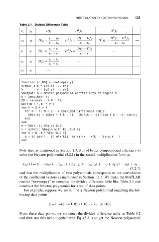
Table 3.1 Divided Difference Table
2 3
x k y k Df k D f k D f k —
2 2
y 1 − y 0 2 Df 1 − Df 0 3 D f 1 − D f 0
x 0 y 0 Df 0 = D f 0 = D f 0 = —
x 1 − x 0 x 2 − x 0 x 3 − x 0
y 2 − y 1 2 Df 2 − Df 1
x 1 y 1 Df 1 = D f 1 = —
x 2 − x 1 x 3 − x 1
y 3 − y 2
x 2 y 2 Df 2 = —
x 3 − x 2
x 3 y 3 —

function [n,DD] = newtonp(x,y)
%Input:x=[x0 x1 ... xN]
% y = [y0 y1 ... yN]
%Output: n = Newton polynomial coefficients of degree N
N = length(x)-1;
DD = zeros(N + 1,N + 1);
DD(1:N + 1,1) = y’;
fork=2:N+1
form=1:N+2-k %Divided Difference Table
DD(m,k) = (DD(m + 1,k - 1) - DD(m,k - 1))/(x(m + k - 1)- x(m));
end
end
a = DD(1,:); %Eq.(3.2.6)
n = a(N+1); %Begin with Eq.(3.2.7)
for k = N:-1:1 %Eq.(3.2.7)
n = [n a(k)] - [0 n*x(k)]; %n(x)*(x - x(k - 1))+a_k - 1
end

Note that, as mentioned in Section 1.3, it is of better computational efficiency to
write the Newton polynomial (3.2.1) in the nested multiplication form as

n N (x) = ((··· (a N (x − x N−1 ) + a N−1 )(x − x N−2 ) +· · ·) + a 1 )(x − x 0 ) + a 0
(3.2.7)
and that the multiplication of two polynomials corresponds to the convolution
of the coefficient vectors as mentioned in Section 1.1.6. We make the MATLAB
routine “newtonp()” to compose the divided difference table like Table 3.1 and
construct the Newton polynomial for a set of data points.
For example, suppose we are to find a Newton polynomial matching the fol-
lowing data points

{(−2, −6), (−1, 0), (1, 0), (2, 6), (4, 60)}

From these data points, we construct the divided difference table as Table 3.2
and then use this table together with Eq. (3.2.1) to get the Newton polynomial