Page 133 - Applied Numerical Methods Using MATLAB

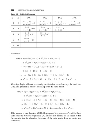
122 INTERPOLATION AND CURVE FITTING
Table 3.2 Divided differences
2 3 4
x k y k Df k D f k D f k D f k
0 − (−6) 0 − 6 2 − (−2) 1 − 1
−2 −6 = 6 =−2 = 1 = 0
−1 − (−2) 1 − (−2) 2 − (−2) 4 − (−2)
0 − 0 6 − 0 7 − 2
−1 0 = 0 = 2 = 1
1 − (−1) 2 − (−1) 4 − (−1)
6 − 0 27 − 6
1 0 = 6 = 7
2 − 1 4 − 1
60 − 6
2 6 = 27
4 − 2
4 60

as follows:
2
n(x) = y 0 + Df 0 (x − x 0 ) + D f 0 (x − x 0 )(x − x 1 )
3
+ D f 0 (x − x 0 )(x − x 1 )(x − x 2 ) + 0
=−6 + 6(x − (−2)) − 2(x − (−2))(x − (−1))
+ 1(x − (−2))(x − (−1))(x − 1)
2
=−6 + 6(x + 2) − 2(x + 2)(x + 1) + (x + 2)(x − 1)
3 2 3
= x + (−2 + 2)x + (6 − 6 − 1)x − 6 + 12 − 4 − 2 = x − x
We might begin with not necessarily the first data point, but, say, the third one
(1,0), and proceed as follows to end up with the same result.

2
n(x) = y 2 + Df 2 (x − x 2 ) + D f 2 (x − x 2 )(x − x 3 )
3
+ D f 2 (x − x 2 )(x − x 3 )(x − x 4 ) + 0
= 0 + 6(x − 1) + 7(x − 1)(x − 2) + 1(x − 1)(x − 2)(x − 4)

2 2
= 6(x − 1) + 7(x − 3x + 2) + (x − 3x + 2)(x − 4)
3 2 3
= x + (7 − 7)x + (6 − 21 + 14)x − 6 + 14 − 8 = x − x
This process is cast into the MATLAB program “do_newtonp.m”, which illus-
trates that the Newton polynomial (3.2.1) does not depend on the order of the
data points; that is, changing the order of the data points does not make any
difference.