Page 130 - Applied Numerical Methods Using MATLAB

INTERPOLATION BY NEWTON POLYNOMIAL 119
6
(2, 6)
4

2
3
(−1, 0) l 3 (x) = x − x (1, 0)
−2 −1 0 1 2
−2

−4
(−2, −6)
−6
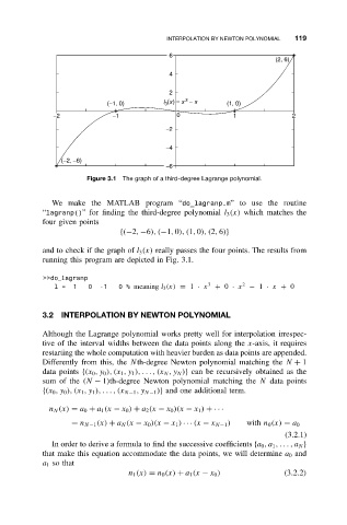
Figure 3.1 The graph of a third-degree Lagrange polynomial.

We make the MATLAB program “do_lagranp.m” to use the routine
“lagranp()” for finding the third-degree polynomial l 3 (x) which matches the
four given points
{(−2, −6), (−1, 0), (1, 0), (2, 6)}

and to check if the graph of l 3 (x) really passes the four points. The results from
running this program are depicted in Fig. 3.1.

>>do lagranp
l= 1 0 -1 0% meaning l 3 (x) = 1 · x 3 + 0 · x 2 − 1 · x + 0

3.2 INTERPOLATION BY NEWTON POLYNOMIAL
Although the Lagrange polynomial works pretty well for interpolation irrespec-
tive of the interval widths between the data points along the x-axis, it requires
restarting the whole computation with heavier burden as data points are appended.
Differently from this, the Nth-degree Newton polynomial matching the N + 1
data points {(x 0 ,y 0 ), (x 1 ,y 1 ), . . . , (x N ,y N )} can be recursively obtained as the
sum of the (N − 1)th-degree Newton polynomial matching the N data points
{(x 0 ,y 0 ), (x 1 ,y 1 ), ...,(x N−1 ,y N−1 )} and one additional term.

n N (x) = a 0 + a 1 (x − x 0 ) + a 2 (x − x 0 )(x − x 1 ) +· · ·
= n N−1 (x) + a N (x − x 0 )(x − x 1 ) ·· · (x − x N−1 ) with n 0 (x) = a 0
(3.2.1)
In order to derive a formula to find the successive coefficients {a 0 ,a 1 ,... ,a N }
that make this equation accommodate the data points, we will determine a 0 and
a 1 so that
n 1 (x) = n 0 (x) + a 1 (x − x 0 ) (3.2.2)