Page 134 - Applied Numerical Methods Using MATLAB

INTERPOLATION BY NEWTON POLYNOMIAL 123

%do_newtonp.m
x = [-2 -1 1 2 4]; y = [-6 0 0 6 60];
n = newtonp(x,y) %l = lagranp(x,y) for comparison
x=[-1 -2 1 2 4]; y=[0-606 60];
n1 = newtonp(x,y) %with the order of data changed for comparison
xx = [-2:0.02: 2]; yy = polyval(n,xx);
clf, plot(xx,yy,’b-’,x,y,’*’)

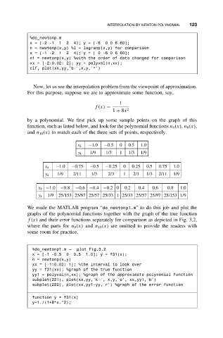
Now, let us see the interpolation problem from the viewpoint of approximation.
For this purpose, suppose we are to approximate some function, say,

1
f(x) =
1 + 8x 2
by a polynomial. We first pick up some sample points on the graph of this
function, such as listed below, and look for the polynomial functions n 4 (x), n 8 (x),
and n 10 (x) to match each of the three sets of points, respectively.

−1.0 −0.5 0 0.5 1.0
x k
1/9 1/3 1 1/3 1/9
y k
−1.0 −0.75 −0.5 −0.25 0 0.25 0.5 0.75 1.0
x k
1/9 2/11 1/3 2/3 1 2/3 1/3 2/11 1/9
y k

x k −1.0 −0.8 −0.6 −0.4 −0.2 0 0.2 0.4 0.6 0.8 1.0
1/9 25/153 25/97 25/57 25/33 1 25/33 25/57 25/97 25/153 1/9
y k
We made the MATLAB program “do_newtonp1.m” todothisjob andplotthe
graphs of the polynomial functions together with the graph of the true function
f(x) and their error functions separately for comparison as depicted in Fig. 3.2,
where the parts for n 8 (x) and n 10 (x) are omitted to provide the readers with
some room for practice.

%do_newtonp1.m – plot Fig.3.2
x = [-1 -0.5 0 0.5 1.0]; y = f31(x);
n = newtonp(x,y)
xx = [-1:0.02: 1]; %the interval to look over
yy = f31(xx); %graph of the true function
yy1 = polyval(n,xx); %graph of the approximate polynomial function
subplot(221), plot(xx,yy,’k-’, x,y,’o’, xx,yy1,’b’)
subplot(222), plot(xx,yy1-yy,’r’) %graph of the error function

function y = f31(x)
y=1./(1+8*x.^2);