Page 139 - Applied Numerical Methods Using MATLAB

128 INTERPOLATION AND CURVE FITTING
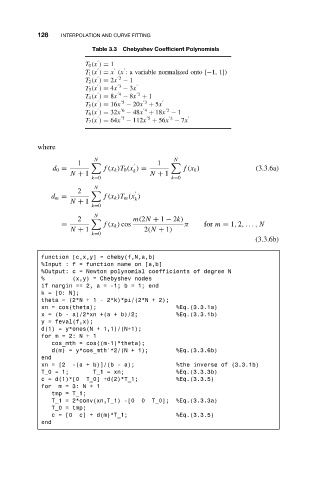
Table 3.3 Chebyshev Coefficient Polynomials

T 0 (x ) = 1

T 1 (x ) = x (x : a variable normalized onto [−1, 1])
2
T 2 (x ) = 2x − 1
3
T 3 (x ) = 4x − 3x
4 2
T 4 (x ) = 8x − 8x + 1

5
3

T 5 (x ) = 16x − 20x + 5x
6

4

2

T 6 (x ) = 32x − 48x + 18x − 1
7

5

3
T 7 (x ) = 64x − 112x + 56x − 7x
where
N N
1 1
d 0 = f(x k )T 0 (x ) = f(x k ) (3.3.6a)
k
N + 1 N + 1
k=0 k=0
N
2
d m = f(x k )T m (x )
k
N + 1
k=0
N
2 m(2N + 1 − 2k)
= f(x k ) cos π for m = 1, 2,..., N
N + 1 2(N + 1)
k=0
(3.3.6b)
function [c,x,y] = cheby(f,N,a,b)
%Input:f= function name on [a,b]
%Output: c = Newton polynomial coefficients of degree N
% (x,y) = Chebyshev nodes
if nargin == 2, a = -1;b=1;end
k = [0: N];
theta = (2*N+1- 2*k)*pi/(2*N + 2);
xn = cos(theta); %Eq.(3.3.1a)
x = (b - a)/2*xn +(a + b)/2; %Eq.(3.3.1b)
y = feval(f,x);
d(1) = y*ones(N + 1,1)/(N+1);
form=2:N+1
cos_mth = cos((m-1)*theta);
d(m) = y*cos_mth’*2/(N + 1); %Eq.(3.3.6b)
end
xn = [2 -(a + b)]/(b - a); %the inverse of (3.3.1b)
T_0 = 1; T_1 = xn; %Eq.(3.3.3b)
c = d(1)*[0 T_0] +d(2)*T_1; %Eq.(3.3.5)
for m=3:N+1
tmp = T_1;
T_1 = 2*conv(xn,T_1) -[0 0 T_0]; %Eq.(3.3.3a)
T_0 = tmp;
c = [0 c] + d(m)*T_1; %Eq.(3.3.5)
end