Page 137 - Applied Numerical Methods Using MATLAB

126 INTERPOLATION AND CURVE FITTING
1.25 0.3
1 0.2 c 4 (x) − f(x)
f(x)
c 4 (x): 0.1
c 8 (x) − f(x)
c 10 (x):
0.5 0
−0.5 0 0.5
c 8 (x): −0.1 c 10 (x) − f(x)
0 −0.2
−0.5 0 0.5
−0.25 −0.3
th
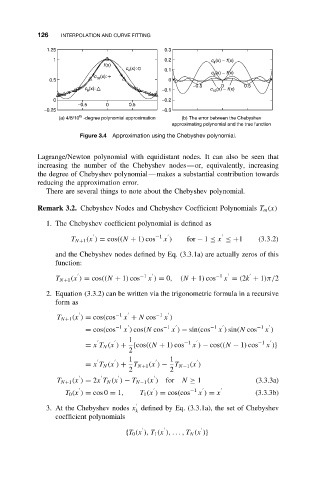
(a) 4/8/10 -degree polynomial approximation (b) The error between the Chebyshev
approximating polynomial and the true function
Figure 3.4 Approximation using the Chebyshev polynomial.

Lagrange/Newton polynomial with equidistant nodes. It can also be seen that
increasing the number of the Chebyshev nodes—or, equivalently, increasing
the degree of Chebyshev polynomial—makes a substantial contribution towards
reducing the approximation error.
There are several things to note about the Chebyshev polynomial.

Remark 3.2. Chebyshev Nodes and Chebyshev Coefficient Polynomials T m (x)
1. The Chebyshev coefficient polynomial is defined as

−1
T N+1 (x ) = cos((N + 1) cos x ) for − 1 ≤ x ≤+1 (3.3.2)
and the Chebyshev nodes defined by Eq. (3.3.1a) are actually zeros of this
function:

−1 −1
T N+1 (x ) = cos((N + 1) cos x ) = 0, (N + 1) cos x = (2k + 1)π/2
2. Equation (3.3.2) can be written via the trigonometric formula in a recursive
form as
−1 −1
T N+1 (x ) = cos(cos x + N cos x )

= cos(cos −1 x ) cos(N cos −1 x ) − sin(cos −1 x ) sin(N cos −1 x )
1
−1 −1
= x T N (x ) + {cos((N + 1) cos x ) − cos((N − 1) cos x )}
2
1 1

= x T N (x ) + T N+1 (x ) − T N−1 (x )
2 2

T N+1 (x ) = 2x T N (x ) − T N−1 (x ) for N ≥ 1 (3.3.3a)
−1
T 0 (x ) = cos 0 = 1, T 1 (x ) = cos(cos x ) = x (3.3.3b)

3. At the Chebyshev nodes x defined by Eq. (3.3.1a), the set of Chebyshev
k
coefficient polynomials

{T 0 (x ), T 1 (x ), ...,T N (x )}