Page 136 - Applied Numerical Methods Using MATLAB

APPROXIMATION BY CHEBYSHEV POLYNOMIAL 125

5p/10

3p/10
p/10
−1 1
x ′ = x ′ = 0 x ′ = x ′ =
1
4
3
0
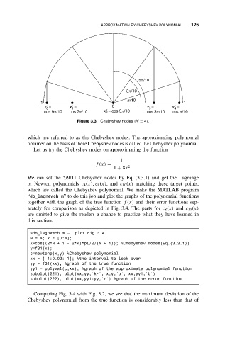
cos 9p/10 cos 7p/10 x ′ = cos 5p/10 cos 3p/10 cos p/10
2
Figure 3.3 Chebyshev nodes (N = 4).
which are referred to as the Chebyshev nodes. The approximating polynomial
obtained on the basis of these Chebyshev nodes is called the Chebyshev polynomial.
Let us try the Chebyshev nodes on approximating the function

1
f(x) =
1 + 8x 2
We can set the 5/9/11 Chebyshev nodes by Eq. (3.3.1) and get the Lagrange
or Newton polynomials c 4 (x), c 8 (x),and c 10 (x) matching these target points,
which are called the Chebyshev polynomial. We make the MATLAB program
“do_lagnewch.m” to do this job and plot the graphs of the polynomial functions
together with the graph of the true function f(x) and their error functions sep-
arately for comparison as depicted in Fig. 3.4. The parts for c 8 (x) and c 10 (x)
are omitted to give the readers a chance to practice what they have learned in
this section.

%do_lagnewch.m – plot Fig.3.4
N = 4; k = [0:N];
x=cos((2*N+1- 2*k)*pi/2/(N + 1)); %Chebyshev nodes(Eq.(3.3.1))
y=f31(x);
c=newtonp(x,y) %Chebyshev polynomial
xx = [-1:0.02: 1]; %the interval to look over
yy = f31(xx); %graph of the true function
yy1 = polyval(c,xx); %graph of the approximate polynomial function
subplot(221), plot(xx,yy,’k-’, x,y,’o’, xx,yy1,’b’)
subplot(222), plot(xx,yy1-yy,’r’) %graph of the error function

Comparing Fig. 3.4 with Fig. 3.2, we see that the maximum deviation of the
Chebyshev polynomial from the true function is considerably less than that of