Page 135 - Applied Numerical Methods Using MATLAB

124 INTERPOLATION AND CURVE FITTING

1
10
f(x) 0.5 n (x) − f(x)
n (x):
0.5 10
0
−0.5 0 0.5
n (x): O n (x) − f(x)
4
0 4
−0.5 0 0.5 −0.5 n (x) − f(x)
8
n (x):
8
th
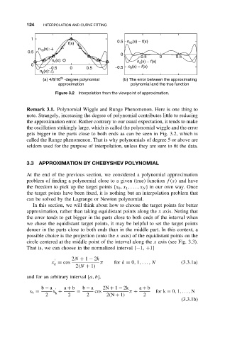
(a) 4/8/10 -degree polynomial (b) The error between the approximating
approximation polynomial and the true function
Figure 3.2 Interpolation from the viewpoint of approximation.
Remark 3.1. Polynomial Wiggle and Runge Phenomenon. Here is one thing to
note. Strangely, increasing the degree of polynomial contributes little to reducing
the approximation error. Rather contrary to our usual expectation, it tends to make
the oscillation strikingly large, which is called the polynomial wiggle and the error
gets bigger in the parts close to both ends as can be seen in Fig. 3.2, which is
called the Runge phenomenon. That is why polynomials of degree 5 or above are
seldom used for the purpose of interpolation, unless they are sure to fit the data.

3.3 APPROXIMATION BY CHEBYSHEV POLYNOMIAL
At the end of the previous section, we considered a polynomial approximation
problem of finding a polynomial close to a given (true) function f(x) and have
the freedom to pick up the target points {x 0 ,x 1 ,...,x N } in our own way. Once
the target points have been fixed, it is nothing but an interpolation problem that
can be solved by the Lagrange or Newton polynomial.
In this section, we will think about how to choose the target points for better
approximation, rather than taking equidistant points along the x axis. Noting that
the error tends to get bigger in the parts close to both ends of the interval when
we chose the equidistant target points, it may be helpful to set the target points
denser in the parts close to both ends than in the middle part. In this context, a
possible choice is the projection (onto the x axis) of the equidistant points on the
circle centered at the middle point of the interval along the x axis (see Fig. 3.3).
That is, we can choose in the normalized interval [−1, +1]

2N + 1 − 2k

x = cos π for k = 0, 1,..., N (3.3.1a)
k
2(N + 1)
and for an arbitrary interval [a, b],
b − a a + b b − a 2N + 1 − 2k a + b
x k = x + = cos π + for k = 0, 1,... , N
k
2 2 2 2(N + 1) 2
(3.3.1b)