Page 138 - Applied Numerical Methods Using MATLAB

APPROXIMATION BY CHEBYSHEV POLYNOMIAL 127
are orthogonal in the sense that
N

T m (x )T n (x ) = 0 for m = n (3.3.4a)
k k
k=0
N
N + 1
2
T (x ) = for m = 0 (3.3.4b)
m k 2
k=0
N
2
T (x ) = N + 1 for m = 0 (3.3.4c)
0 k
k=0

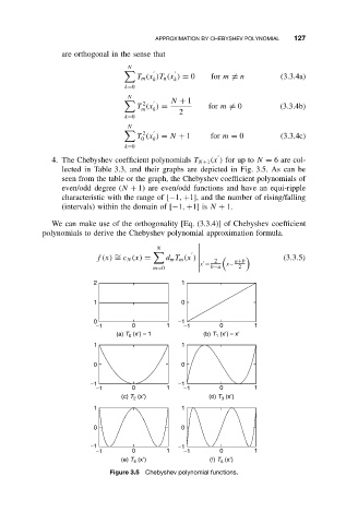
4. The Chebyshev coefficient polynomials T N+1 (x ) for up to N = 6are col-
lected in Table 3.3, and their graphs are depicted in Fig. 3.5. As can be
seen from the table or the graph, the Chebyshev coefficient polynomials of
even/odd degree (N + 1) are even/odd functions and have an equi-ripple
characteristic with the range of [−1, +1], and the number of rising/falling
(intervals) within the domain of [−1, +1] is N + 1.

We can make use of the orthogonality [Eq. (3.3.4)] of Chebyshev coefficient
polynomials to derive the Chebyshev polynomial approximation formula.

N

∼
f(x) = c N (x) = d m T m (x ) 2 (3.3.5)
a+b
x = x−
m=0 b−a 2
2 1
1 0

0 −1
−1 0 1 −1 0 1
(a) T 0 (x′) = 1 (b) T 1 (x′) = x′
1 1

0 0

−1 −1
−1 0 1 −1 0 1
(c) T 2 (x′) (d) T 3 (x′)
1 1

0 0
−1 −1
−1 0 1 −1 0 1
(e) T 4 (x′) (f) T 5 (x′)
Figure 3.5 Chebyshev polynomial functions.