Page 143 - Applied Numerical Methods Using MATLAB

132 INTERPOLATION AND CURVE FITTING
1

0.5

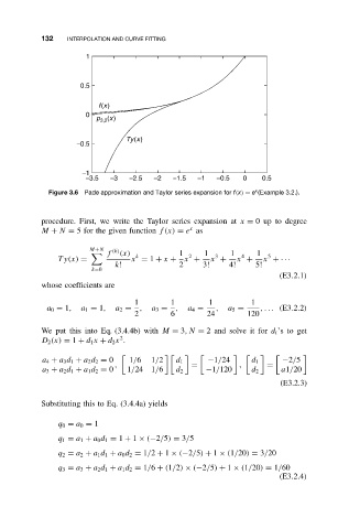
f(x)
0
p 3,2 (x)

Ty(x)
−0.5

−1
−3.5 −3 −2.5 −2 −1.5 −1 −0.5 0 0.5
x
Figure 3.6 Pade approximation and Taylor series expansion for f(x) = e (Example 3.2.).

procedure. First, we write the Taylor series expansion at x = 0up todegree
x
M + N = 5 for the given function f(x) = e as
M+N (k)
f (x) k 1 2 1 3 1 4 1 5
Ty(x) = x = 1 + x + x + x + x + x +· · ·
k! 2 3! 4! 5!
k=0
(E3.2.1)
whose coefficients are
1 1 1 1
a 0 = 1, a 1 = 1, a 2 = , a 3 = , a 4 = , a 5 = ,... (E3.2.2)
2 6 24 120

We put this into Eq. (3.4.4b) with M = 3,N = 2 and solve it for d i ’s to get
2
D 2 (x) = 1 + d 1 x + d 2 x .

a 4 + a 3 d 1 + a 2 d 2 = 0 1/6 1/2 d 1 −1/24 d 1 −2/5
, = , =
a 3 + a 2 d 1 + a 1 d 2 = 0 1/24 1/6 d 2 −1/120 d 2 a1/20
(E3.2.3)

Substituting this to Eq. (3.4.4a) yields

q 0 = a 0 = 1
q 1 = a 1 + a 0 d 1 = 1 + 1 × (−2/5) = 3/5

q 2 = a 2 + a 1 d 1 + a 0 d 2 = 1/2 + 1 × (−2/5) + 1 × (1/20) = 3/20
q 3 = a 3 + a 2 d 1 + a 1 d 2 = 1/6 + (1/2) × (−2/5) + 1 × (1/20) = 1/60
(E3.2.4)