Page 147 - Applied Numerical Methods Using MATLAB

136 INTERPOLATION AND CURVE FITTING
and, subsequently, we have just N − 1 unknowns. In the case where the second-
order derivatives on the two boundary points are given as (iii) in Table 3.4

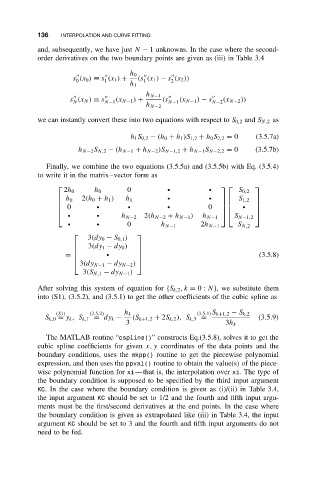
h 0

s (x 0 ) ≡ s (x 1 ) + (s (x 1 ) − s (x 2 ))
1
0
1
2
h 1
h N−1

s (x N ) ≡ s (x N−1 ) + (s (x N−1 ) − s (x N−2 ))
N N−1 N−1 N−2
h N−2
we can instantly convert these into two equations with respect to S 0,2 and S N,2 as
h 1 S 0,2 − (h 0 + h 1 )S 1,2 + h 0 S 2,2 = 0 (3.5.7a)
h N−2 S N,2 − (h N−1 + h N−2 )S N−1,2 + h N−1 S N−2,2 = 0 (3.5.7b)
Finally, we combine the two equations (3.5.5a) and (3.5.5b) with Eq. (3.5.4)
to write it in the matrix–vector form as

 0 ž ž   
2h 0 h 0 S 0,2
2(h 0 + h 1 ) ž ž
 h 0 h 1   S 1,2 
 0 ž ž ž 0   ž 

 

ž ž h N−2 2(h N−2 + h N−1 ) h N−1 S N−1,2
   
ž ž 0 h N−1 2h N−1 S N,2
3(dy 0 − S 0,1 )
 
3(dy 1 − dy 0 )
 
 
ž (3.5.8)
= 

3(dy N−1 − dy N−2 )
 
3(S N,1 − dy N−1 )
After solving this system of equation for {S k,2 ,k = 0: N}, we substitute them
into (S1), (3.5.2), and (3.5.1) to get the other coefficients of the cubic spline as
(S1) (3.5.2) h k (3.5.1)S k+1,2 − S k,2
S k,0 = y k ,S k,1 = dy k − (S k+1,2 + 2S k,2 ), S k,3 = (3.5.9)
3 3h k
The MATLAB routine “cspline()” constructs Eq.(3.5.8), solves it to get the
cubic spline coefficients for given x, y coordinates of the data points and the
boundary conditions, uses the mkpp() routine to get the piecewise polynomial
expression, and then uses the ppval() routine to obtain the value(s) of the piece-
wise polynomial function for xi—that is, the interpolation over xi. The type of
the boundary condition is supposed to be specified by the third input argument
KC. In the case where the boundary condition is given as (i)/(ii) in Table 3.4,
the input argument KC should be set to 1/2 and the fourth and fifth input argu-
ments must be the first/second derivatives at the end points. In the case where
the boundary condition is given as extrapolated like (iii) in Table 3.4, the input
argument KC should be set to 3 and the fourth and fifth input arguments do not
need to be fed.