Page 150 - Applied Numerical Methods Using MATLAB

HERMITE INTERPOLATING POLYNOMIAL 139

5

4
3

2

1
0
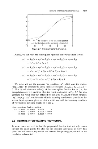
: 1st derivatives on the end points specified
: 2nd derivatives on the end points extrapolated
−1
0 0.5 1 1.5 2 2.5 3
Figure 3.7 Cubic splines for Example 3.3.

Finally, we can write the cubic spline equations collectively from (S0) as
3 2
s 0 (x) = S 0,3 (x − x 0 ) + S 0,2 (x − x 0 ) + S 0,1 (x − x 0 ) + S 0,0
3
2
= 2x − 3x + 2x + 0
3 2
s 1 (x) = S 1,3 (x − x 1 ) + S 1,2 (x − x 1 ) + S 1,1 (x − x 1 ) + S 1,0
2
3
=−2(x − 1) + 3(x − 1) + 2(x − 1) + 1
3 2
s 2 (x) = S 2,3 (x − x 2 ) + S 2,2 (x − x 2 ) + S 2,1 (x − x 2 ) + S 2,0
2
3
= 2(x − 2) − 3(x − 2) + 2(x − 1) + 4
We make and run the program “do_csplines.m”, which uses the routine
“cspline()” to compute the cubic spline coefficients {S k,3 ,S k,2 ,S k,1 ,S k,0 ,k =
0: N − 1} and obtain the value(s) of the cubic spline function for xi (i.e., the
interpolation over xi) and then plots the result as depicted in Fig. 3.7. We also
compare this result with that obtained by using the MATLAB built-in function
“spline(x,y,xi)”, which works with the boundary condition of type (i) for the
second input argument given as [dy0 y dyN], and with the boundary condition
of type (iii) for the same lengths of x and y.

>>do_csplines %cubic spline
S = 2.0000 -3.0000 2.0000 0
-2.0000 3.0000 2.0000 1.0000
2.0000 -3.0000 2.0000 4.0000

3.6 HERMITE INTERPOLATING POLYNOMIAL

In some cases, we need to find the polynomial function that not only passes
through the given points, but also has the specified derivatives at every data
point. We call such a polynomial the Hermite interpolating polynomial or the
osculating polynomial.