Page 154 - Applied Numerical Methods Using MATLAB

CURVE FITTING 143

%do_interp2.m
% 2-dimensional interpolation for Ex 3.5
xi = -2:0.1:2; yi = -2:0.1:2;
[Xi,Yi] = meshgrid(xi,yi);
Z0 = Xi.^2 + Yi.^2; %(E3.5.1)
subplot(131), mesh(Xi,Yi,Z0)
x = -2:0.5:2; y = -2:0.5:2;
[X,Y] = meshgrid(x,y);
Z = X.^2 + Y.^2;
subplot(132), mesh(X,Y,Z)
Zi = interp2(x,y,Z,Xi,Yi); %built-in routine
subplot(133), mesh(xi,yi,Zi)
Zi = intrp2(x,y,Z,xi,yi); %our own routine
pause, mesh(xi,yi,Zi)
norm(Z0 - Zi)/norm(Z0)

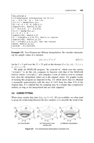
Example 3.5. Two-Dimensional Bilinear Interpolation. We consider interpolat-
ing the sample values of a function
2
f (x, y) = x + y 2 (E3.5.1)
for the 5 × 5 grid over the 21 × 21 grid on the domain D ={(x, y)|− 2 ≤ x ≤
2, −2 ≤ y ≤ 2}.
We make the MATLAB program “do_interp2.m”, which uses the routine
“intrp2()” to do this job, compares its function with that of the MATLAB
built-in routine “interp2()”, and computes a kind of relative error to estimate
how close the interpolated values are to the original values. The graphic results
of running this program are depicted in Fig. 3.9, which shows that we obtained
a reasonable approximation with the error of 2.6% from less than 1/16 of the
original data. It is implied that the sampling may be a simple data compression
method, as long as the interpolated data are little impaired.

3.8 CURVE FITTING
When many sample data pairs {(x k ,y k ), k = 0: M} are available, we often need
to grasp the relationship between the two variables or to describe the trend of the

10 10 10

5 5 5
0 0 0
2 2 2 2 2 2
0 0 0 0 0 0
−2 −2 −2 −2 −2 −2
(a) True function (b) The function over (c) Bilinear interpolation
sample grid

Figure 3.9 Two-dimensional interpolation (Example 3.5).