Page 155 - Applied Numerical Methods Using MATLAB

144 INTERPOLATION AND CURVE FITTING
data, hopefully in a form of function y = f(x). But, as mentioned in Remark 3.1,
the polynomial approach meets with the polynomial wiggle and/or Runge phe-
nomenon, which makes it not attractive for approximation purpose. Although the
cubic spline approach may be a roundabout toward the smoothness as explained
in Section 3.5, it has too many parameters and so does not seem to be an effi-
cient way of describing the relationship or the trend, since every subinterval
needs four coefficients. What other choices do we have? Noting that many data
are susceptible to some error, we don’t have to try to find a function passing
exactly through every point. Instead of pursuing the exact matching at every data
point, we look for an approximate function (not necessarily a polynomial) that
describes the data points as a whole with the smallest error in some sense, which
is called the curve fitting.
As a reasonable means, we consider the least-squares (LS) approach to min-
imizing the sum of squared errors, where the error is described by the vertical
distance to the curve from the data points. We will look over various types of
fitting functions in this section.

3.8.1 Straight Line Fit: A Polynomial Function of First Degree
If there is some theoretical basis on which we believe the relationship between
the two variables to be
θ 1 x + θ 0 = y (3.8.1)

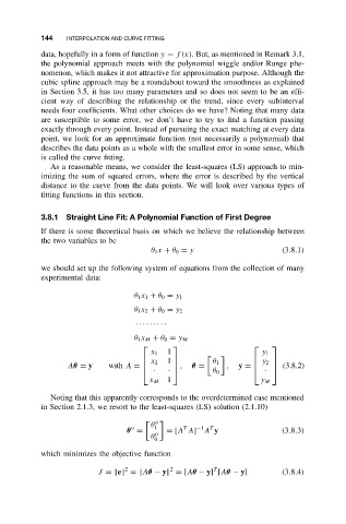
we should set up the following system of equations from the collection of many
experimental data:

θ 1 x 1 + θ 0 = y 1
θ 1 x 2 + θ 0 = y 2
· · ·· ···· ·

θ 1 x M + θ 0 = y M
   
x 1 1 y 1

 x 2 1  θ 1  
Aθ = y with A =   , θ = , y =  y 2  (3.8.2)
 · θ 0  · 
· 
x M 1 y M
Noting that this apparently corresponds to the overdetermined case mentioned
in Section 2.1.3, we resort to the least-squares (LS) solution (2.1.10)

θ
o
o 1 T −1 T
θ = o = [A A] A y (3.8.3)
θ
0
which minimizes the objective function
2
2
T
J =||e|| =||Aθ − y|| = [Aθ − y] [Aθ − y] (3.8.4)