Page 160 - Applied Numerical Methods Using MATLAB

CURVE FITTING 149
(cf) Note that the objective of the WLS scheme is to put greater emphasis on more
reliable data.

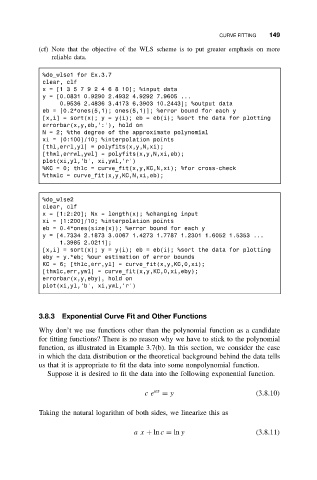
%do_wlse1 for Ex.3.7
clear, clf
x=[135792468 10]; %input data
y = [0.0831 0.9290 2.4932 4.9292 7.9605 ...
0.9536 2.4836 3.4173 6.3903 10.2443]; %output data
eb = [0.2*ones(5,1); ones(5,1)]; %error bound for each y
[x,i] = sort(x); y = y(i); eb = eb(i); %sort the data for plotting
errorbar(x,y,eb,’:’), hold on
N = 2; %the degree of the approximate polynomial
xi = [0:100]/10; %interpolation points
[thl,errl,yl] = polyfits(x,y,N,xi);
[thwl,errwl,ywl] = polyfits(x,y,N,xi,eb);
plot(xi,yl,’b’, xi,ywl,’r’)
%KC = 0; thlc = curve_fit(x,y,KC,N,xi); %for cross-check
%thwlc = curve_fit(x,y,KC,N,xi,eb);

%do_wlse2
clear, clf
x = [1:2:20]; Nx = length(x); %changing input
xi = [1:200]/10; %interpolation points
eb = 0.4*ones(size(x)); %error bound for each y
y = [4.7334 2.1873 3.0067 1.4273 1.7787 1.2301 1.6052 1.5353 ...
1.3985 2.0211];
[x,i] = sort(x); y = y(i); eb = eb(i); %sort the data for plotting
eby = y.*eb; %our estimation of error bounds
KC = 6; [thlc,err,yl] = curve_fit(x,y,KC,0,xi);
[thwlc,err,ywl] = curve_fit(x,y,KC,0,xi,eby);
errorbar(x,y,eby), hold on
plot(xi,yl,’b’, xi,ywl,’r’)

3.8.3 Exponential Curve Fit and Other Functions

Why don’t we use functions other than the polynomial function as a candidate
for fitting functions? There is no reason why we have to stick to the polynomial
function, as illustrated in Example 3.7(b). In this section, we consider the case
in which the data distribution or the theoretical background behind the data tells
us that it is appropriate to fit the data into some nonpolynomial function.
Suppose it is desired to fit the data into the following exponential function.

ce ax = y (3.8.10)

Taking the natural logarithm of both sides, we linearize this as

ax + ln c = ln y (3.8.11)