Page 161 - Applied Numerical Methods Using MATLAB

150 INTERPOLATION AND CURVE FITTING
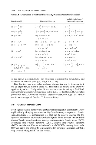
Table 3.5 Linearization of Nonlinear Functions by Parameter/Data Transformation

Variable Substitution/
Function to Fit Linearized Function Parameter Restoration
a 1 1

(1) y = + b y = a + b → y = ax + b x =
x x x
b 1 1 a 1 b 1

(2) y = = x + → y = a x + b y = ,a = ,b =
x + a y b b y a a

b
(3) y = ab x ln y = (ln b)x + ln a y = ln y, a = e ,b = e a

→ y = a x + b

(4) y = be ax ln y = ax + ln b → y = ax + b y = ln y, b = e b

(5) y = C − be −ax ln(C − y) =−ax + ln b y = ln(C − y)

→ y = a x + b a =−a ,b = e b

(6) y = ax b ln y = b(ln x) + ln a y = ln y, x = ln x
b

→ y = a x + b a = e ,b = a

(7) y = ax e bx ln y − ln x = bx + ln a y = ln(y/x)
b

→ y = a x + b a = e ,b = a

C C C

(8) y = ln − 1 = ax + ln b y = ln − 1 ,b = e b
1 + be ax y y

(a 0,b 0,C = y(∞)) → y = ax + b
(9) y = a ln x + b → y = ax + b x = ln x

so that the LS algorithm (3.8.3) can be applied to estimate the parameters a and
ln c based on the data pairs {(x k , ln y k ), k = 0: M}.
Like this, there are many other nonlinear relations that can be linearized to fit
the LS algorithm, as listed in Table 3.5. This makes us believe in the extensive
applicability of the LS algorithm. If you are interested in making a MATLAB
routine that implements what are listed in this table, see Problem 3.11, which lets
you try the MATLAB built-in function “lsqcurvefit(f,th0,x,y)” that enables
one to use any type of function (f) for curve fitting.
3.9 FOURIER TRANSFORM
Most signals existent in this world contain various frequency components, where
rapidly/slowly changing one contains high/low-frequency components. Fourier
series/transform is a mathematical tool that can be used to analyze the fre-
quency characteristic of periodic/aperiodic signals. There are four similar defini-
tions of Fourier series/transform, namely, continuous-time Fourier series (CtFS),
continuous-time Fourier transform (CtFT), discrete-time Fourier transform
(DtFT), and discrete Fourier series/transform (DFS/DFT). Among these tools,
DFT can easily and efficiently be programmed in computer languages and that’s
why we deal with just DFT in this section.