Page 166 - Applied Numerical Methods Using MATLAB

FOURIER TRANSFORM 155
blurred like this is said to be the ‘leakage problem’. The leakage problem occurs
in most cases because we cannot determine the length of the whole time interval
in such a way that it is a multiple of the period of the signal as long as we don’t
know in advance the frequency contents of the signal. If we knew the frequency
contents of a signal, why do we bother to find its spectrum that is already known?
As a measure to alleviate the leakage problem, there is a windowing technique
[O-1, Section 11.2]. Interested readers can see Problem 3.18.
Also note that the periodicity with period N(the DFT size) of the DFT
sequence X(k) as well as x[n], as can be manifested by substituting k + mN
(m represents any integer) for k in Eq. (3.9.1a) and also substituting n + mN
for n in Eq. (3.9.1b). A real-world example reminding us of the periodicity of
DFT spectrum is the so-called stroboscopic effect whereby the wheel of a car-
riage driven by a horse in the scene of a western movie looks like spinning at
lower speed than its real speed or even in the reverse direction. The periodicity
of x[n] is surprising, because we cannot imagine that every discrete-time signal
is periodic with the period of N, which is the variable size of the DFT to be
determined by us. As a matter of fact, the ‘weird’ periodicity of x[n] can be
regarded as a kind of cost that we have to pay for computing the sampled DFT
spectrum instead of the continuous spectrum X(ω) for a continuous-time signal
x(t), which is originally defined as

∞

X(ω) = x(t)e −jωt dt (3.9.4)
−∞
Actually, this is to blame for the blurred spectra of the two-tone signal depicted
in Fig. 3.13.

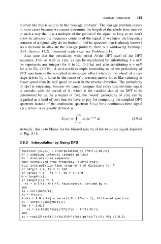
3.9.3 Interpolation by Using DFS

function [xi,Xi] = interpolation_by_DFS(T,x,Ws,ti)
%T : sampling interval (sample period)
%x : discrete-time sequence
%Ws: normalized stop frequency (1.0=pi[rad])
%ti: interpolation time range or # of divisions for T
if nargin < 4, ti = 5; end
if nargin<3|Ws>1, Ws=1;end
N = length(x);
if length(ti) == 1
ti = 0:T/ti:(N-1)*T; %subinterval divided by ti
end
ks = ceil(Ws*N/2);
Xi = fft(x);
Xi(ks + 2:N - ks) = zeros(1,N - 2*ks - 1); %filtered spectrum
xi = zeros(1,length(ti));
for k = 2:N/2
xi = xi+Xi(k)*exp(j*2*pi*(k - 1)*ti/N/T);
end
xi = real(2*xi+Xi(1)+Xi(N/2+1)*cos(pi*ti/T))/N; %Eq.(3.9.5)