Page 171 - Applied Numerical Methods Using MATLAB

160 INTERPOLATION AND CURVE FITTING

k 0 1 2 3 4

x k −π −π/2 0 +π/2 +π
f(x k ) −1 0 1 0 −1

(b) Find the Lagrange/Newton polynomial of degree 4 matching the fol-
lowing five points and plot the resulting polynomial on the same graph
that has the result of (a).

k 0 1 2 3 4
π cos(9π/10)π cos(7π/10) 0 π cos(3π/10)π cos(π/10)
x k
f(x k ) −0.9882 −0.2723 1 −0.2723 −0.9882

(c) Find the Chebyshev polynomial of degree 4 for cos x over [−π, +π]
and plot the resulting polynomial on the same graph that has the result
of (a) and (b).
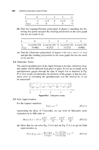
3.4 Chebyshev Nodes
The current speed/pressure of the liquid flowing in the pipe, which has irreg-
ular radius, will be different from place to place. If you are to install seven
speed/pressure gauges through the pipe of length 4 m as depicted in Fig.
P3.4, how would you determine the positions of the gauges so that the max-
imum error of estimating the speed/pressure over the interval [0, 4] can
be minimized?

x
0 1 2 3 4
Figure P3.4 Chebyshev nodes.
3.5 Pade Approximation
For the Laplace transform
F(s) = e −sT (P3.5.1)

representing the delay of T [seconds], we can write its Maclaurin series
expansionuptofifth order as

(sT ) 2 (sT ) 3 (sT ) 4 (sT ) 5
∼
Mc(s) = 1 − sT + − + − (P3.5.2)
2! 3! 4! 5!
(a) Show that we can solve Eq. (3.4.4) and use Eq. (3.4.1) to get the Pade
approximation as
q 0 + q 1 s 1 − (T /2)s
∼ ∼ −Ts
F(s) = p 1,1 (s) = = = e (P3.5.3)
1 + d 1 s 1 + (T /2)s