Page 175 - Applied Numerical Methods Using MATLAB

164 INTERPOLATION AND CURVE FITTING
3.9 Robot Path Planning Using Cubic Spline
Every object having a mass is subject to the law of inertia and so its
speed described by the first derivative of its displacement with respect to
time must be continuous in any direction. In this context, the cubic spline
having the continuous derivatives up to second order presents a good basis
for planning the robot path/trajectory. We will determine the path of a robot
in such a way that the following conditions are satisfied:
ž At time t = 0 s, the robot starts from its home position (0, 0) with zero
initial velocity, passing through the intermediate point (1, 1) at t = 1s
and arriving at the final point (2, 4) at t = 2s.
ž On arriving at (2, 4), it starts the point at t = 2 s, stopping by the
intermediate point (3, 3) at t = 3 s and arriving at the point (4, 2) at
t = 4s.
ž On arriving at (4, 2), it starts the point, passing through the intermediate
point (2,1) at t = 5 s and then returning to the home position (0, 0) at
t = 6s.
More specifically, what we need is
ž the spline interpolation matching the three points (0, 0),(1, 1),(2, 2) and
having zero velocity at both boundary points (0, 0) and (2, 2),
ž the spline interpolation matching the three points (2, 2),(3, 3),(4, 4) and
having zero velocity at both boundary points (2, 2) and (4, 4), and
ž the spline interpolation matching the three points (4, 4), (5, 2), (6, 0) and
having zero velocity at both boundary points (4, 4) and (6, 0) on the tx
plane.
On the ty plane, we need
ž the spline interpolation matching the three points (0, 0),(1, 1),(2, 4) and
having zero velocity at both boundary points (0, 0) and (2, 4),
ž the spline interpolation matching the three points (2, 4),(3, 3),(4, 2) and
having zero velocity at both boundary points (2, 4) and (4, 2), and
ž the spline interpolation matching the three points (4, 2),(5, 1),(6, 0) and
having zero velocity at both boundary points (4, 2) and (6, 0).
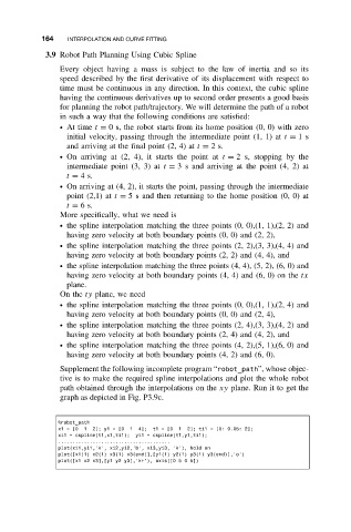
Supplement the following incomplete program “robot_path”, whose objec-
tive is to make the required spline interpolations and plot the whole robot
path obtained through the interpolations on the xy plane. Run it to get the
graph as depicted in Fig. P3.9c.

%robot_path
x1 = [0 1 2]; y1 = [0 1 4]; t1 = [0 1 2]; ti1 = [0: 0.05: 2];
xi1 = cspline(t1,x1,ti1); yi1 = cspline(t1,y1,ti1);
.......................................
plot(xi1,yi1,’k’, xi2,yi2,’b’, xi3,yi3, ’k’), hold on
plot([x1(1) x2(1) x3(1) x3(end)],[y1(1) y2(1) y3(1) y3(end)],’o’)
plot([x1 x2 x3],[y1 y2 y3],’k+’), axis([0505])