Page 176 - Applied Numerical Methods Using MATLAB

PROBLEMS 165
x y y
5 5 5
tx plane ty plane xy plane 2
4 + 4 + 4 +
3 + 3 + 3 + 3
2 + + 2 + 2 + 4
1 + 1 + + 1 1 + +
5
0 + + 0 + + 0 + 0
0 2 4 t 6 0 2 4 t 6 0 1 2 3 4 x 5
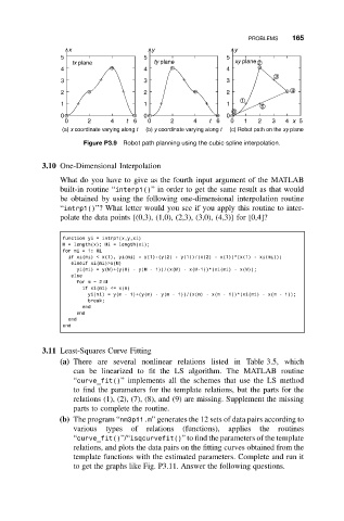
(a) x coordinate varying along t (b) y coordinate varying along t (c) Robot path on the xy plane
Figure P3.9 Robot path planning using the cubic spline interpolation.

3.10 One-Dimensional Interpolation
What do you have to give as the fourth input argument of the MATLAB
built-in routine “interp1()” in order to get the same result as that would
be obtained by using the following one-dimensional interpolation routine
“intrp1()”? What letter would you see if you apply this routine to inter-
polate the data points {(0,3), (1,0), (2,3), (3,0), (4,3)} for [0,4]?

function yi = intrp1(x,y,xi)
M = length(x); Mi = length(xi);
for mi=1:Mi
if xi(mi) < x(1), yi(mi) = y(1)-(y(2) - y(1))/(x(2) - x(1))*(x(1) - xi(mi));
elseif xi(mi)>x(M)
yi(mi) = y(M)+(y(M) - y(M - 1))/(x(M) - x(M-1))*(xi(mi) - x(M));
else
for m = 2:M
if xi(mi) <= x(m)
yi(mi) = y(m - 1)+(y(m) - y(m - 1))/(x(m) - x(m - 1))*(xi(mi) - x(m - 1));
break;
end
end
end
end

3.11 Least-Squares Curve Fitting
(a) There are several nonlinear relations listed in Table 3.5, which
can be linearized to fit the LS algorithm. The MATLAB routine
“curve_fit()” implements all the schemes that use the LS method
to find the parameters for the template relations, but the parts for the
relations (1), (2), (7), (8), and (9) are missing. Supplement the missing
parts to complete the routine.
(b) The program “nm3p11.m” generates the 12 sets of data pairs according to
various types of relations (functions), applies the routines
“curve_fit()”/“lsqcurvefit()” to find the parameters of the template
relations, and plots the data pairs on the fitting curves obtained from the
template functions with the estimated parameters. Complete and run it
to get the graphs like Fig. P3.11. Answer the following questions.