Page 181 - Applied Numerical Methods Using MATLAB

170 INTERPOLATION AND CURVE FITTING
from 1 (see Remark 2.3). You will realize something about this issue after
solving this problem.
6
(a) Find a polynomial of degree 2 which fits four data points (10 , 1), (1.1 ×
6
6
6
10 , 2), (1.2 × 10 ,5), and(1.3 × 10 , 10) and plot the polynomial
6
function (together with the data points) over the interval [10 , 1.3 ×
6
10 ] to check whether it fits the data points well. How big is the relative
mismatch error? Does the polynomial do the fitting job well?
7
(b) Find a polynomial of degree 2 which fits four data points (10 , 1),(1.1 ×
7
7
7
10 , 2), (1.2 × 10 ,5), and(1.3 × 10 , 10) and plot the polynomial
7
function (together with the data points) over the interval [10 , 1.3 ×
7
10 ] to check whether it fits the data points well. How big is the relative
mismatch error? Does the polynomial do the fitting job well? Did you
get any warning message on the MATLAB command window? What
do you think about it?
(c) If you are not satisfied with the result obtained in (b), why don’t you
try the scaled curve fitting scheme described below?
1. Transform the x n ’s of the data point (x n ,y n )’s into the region
[−2, 2] by the following relation.
4

x ←−2 + (x n − x min ) (P3.14.1)
n
x max − x min

2. Find the LS polynomial p(x ) fitting the data point (x , y n )’s.
n
3. Substitute
4

x ←−2 + (x − x min ) (P3.14.2)
x max − x min
for x into p(x ).

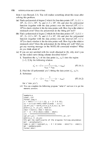
(cf) You can complete the following program “nm3p14”and runittoget the
numeric answers.
%nm3p14.m
clear, clf
format long e
x = 1e6*[1 1.1 1.2 1.3];y=[125 10];
xi = x(1)+[0:1000]/1000*(x(end) - x(1));
[p,err,yi] = curve_fit(x,y,0,2,xi); p, err
plot(x,y,’o’,xi,yi), hold on
xmin = min(x); xmax = max(x);
x1 = -2 + 4*(x-xmin)/(xmax - xmin);
x1i = ??????????????????????????;
[p1,err,yi] = ?????????????????????????; p1, err
plot(x,y,’o’,xi,yi)
%To get the coefficients of the original fitting polynomial
ps1 = poly2sym(p1);
syms x; ps0 = subs(ps1,x,-2+ 4/(xmax - xmin)*(x - xmin));
p0 = sym2poly(ps0)
format short