Page 183 - Applied Numerical Methods Using MATLAB

172 INTERPOLATION AND CURVE FITTING
3.17 Effect of Sampling Period, Zero-Padding, and Whole Time Interval on
DFT Spectrum
In Section 3.9.2, we experienced the effect of zero-padding, sampling period
reduction, and whole interval extension on the DFT spectrum of a two-tone
signal that has two distinct frequency components. Here, we are going
to investigate the effect of zero-padding, sampling period reduction, and
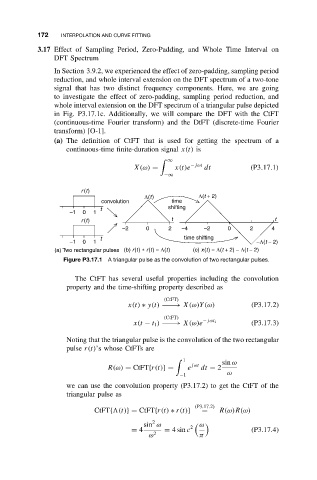
whole interval extension on the DFT spectrum of a triangular pulse depicted
in Fig. P3.17.1c. Additionally, we will compare the DFT with the CtFT
(continuous-time Fourier transform) and the DtFT (discrete-time Fourier
transform) [O-1].
(a) The definition of CtFT that is used for getting the spectrum of a
continuous-time finite-duration signal x(t) is

∞
X(ω) = x(t)e −jωt dt (P3.17.1)
−∞
r (t)
Λ(t) Λ(t + 2)
convolution time
t shifting
–1 0 1
r (t) t t
–2 0 2 –4 –2 0 2 4
t time shifting
–1 0 1 −Λ(t − 2)
(a) Two rectangular pulses (b) r(t) ∗ r(t) = Λ(t) (c) x(t) = Λ(t + 2) − Λ(t − 2)
Figure P3.17.1 A triangular pulse as the convolution of two rectangular pulses.

The CtFT has several useful properties including the convolution
property and the time-shifting property described as

(CtFT)
x(t) ∗ y(t) −−−→ X(ω)Y(ω) (P3.17.2)
(CtFT)
x(t − t 1 ) −−−→ X(ω)e −jωt 1 (P3.17.3)
Noting that the triangular pulse is the convolution of the two rectangular
pulse r(t)’s whose CtFTs are
1 sin ω
R(ω) = CtFT{r(t)}= e jωt dt = 2
−1 ω
we can use the convolution property (P3.17.2) to get the CtFT of the
triangular pulse as
(P3.17.2)
CtFT{ (t)}= CtFT{r(t) ∗ r(t)} = R(ω)R(ω)
2
ω
sin ω 2
= 4 = 4sin c (P3.17.4)
ω 2 π