Page 180 - Applied Numerical Methods Using MATLAB

PROBLEMS 169
(cf) If you have no idea, insert just one statement involving ‘interp2()’into
the program ‘nm1p04.m’ (Problem 1.4) and fit it into the format of a MAT-
LAB function.
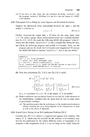
3.13 Polynomial Curve Fitting by Least Squares and Persistent Excitation
Suppose the theoretical (true) relationship between the input x and the
output y is known as
y = x + 2 (P3.13.1)

Charley measured the output data y 10 times for the same input value
x = 1 by using a gauge whose measurement errors has a uniform distribu-
tion U[−0.5, +0.5]. He made the following MATLAB program “nm3p13”,
which uses the routine “polyfits()” to find a straight line fitting the data.
(a) Check the following program and modify it if needed. Then, run the
program and see the result. Isn’t it beyond your imagination? If you use
the MATLAB built-in function “polyfit()”, does it get any better?

%nm3p13.m
tho = [1 2]; %true parameter
x = ones(1,10); %the unchanged input
y = tho(1)*x + tho(2)+(rand(size(x)) - 0.5);
th_ls = polyfits(x,y,1); %uses the MATLAB routine in Sec.3.8.2
polyfit(x,y,1) %uses MATLAB built-in function

(b) Note that substituting Eq. (3.8.2) into Eq.(3.8.3) yields
o
a
o T −1 T
θ = = [A A] A y
b o
M 2 M −1 M

n=0 x n n=0 x n n=0 x n y n
= (P3.13.2)
M M M
n=0 x n n=0 1 n=0 y n
T
If x n = c(constant) ∀ n = 0: M, is the matrix A A invertible?
(c) What conclusion can you derive based on (a) and (b), with reference to
the identifiability condition that the input must be rich in some sense
or persistently exciting?
(cf) This problem implies that the performance of the identification/estimation
scheme including the curve fitting depends on the characteristic of input
as well as the choice of algorithm.
3.14 Scaled Curve Fitting for an Ill-Conditioned Problem [M-2]
Consider Eq. (P3.13.2), which is a typical least-squares (LS) solution. The
T
matrix A A, which must be inverted for the solution to be obtained, may
become ill-conditioned by the widely different orders of magnitude of its
elements, if the magnitudes of all x n ’s are too large or too small, being far