Page 177 - Applied Numerical Methods Using MATLAB

166 INTERPOLATION AND CURVE FITTING
(i) If any, find the case(s) where the results of using the two routines
make a great difference. For the case(s), try with another initial
guess th0 = [1 1] of parameters, instead of th0 = [0 0].
(ii) If the MATLAB built-in routine “lsqcurvefit()” yields a bad
result, does it always give you a warning message? How do you
compare the two routines?

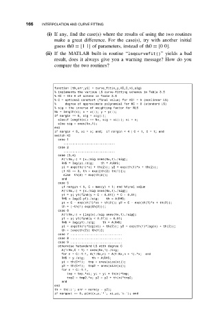
function [th,err,yi] = curve_fit(x,y,KC,C,xi,sig)
% implements the various LS curve-fitting schemes in Table 3.5
% KC = the # of scheme in Table 3.5
% C = optional constant (final value) for KC! = 0 (nonlinear LS)
% degree of approximate polynomial for KC = 0 (standard LS)
% sig = the inverse of weighting factor for WLS
Nx = length(x); x = x(:); y = y(:);
if nargin == 6, sig = sig(:);
elseif length(xi) == Nx, sig = xi(:); xi = x;
else sig = ones(Nx,1);
end
if nargin < 5, xi = x; end; if nargin < 4 | C<1,C=1;end
switch KC
case 1
.............................
case 2
.............................
case {3,4}
A(1:Nx,:) = [x./sig ones(Nx,1)./sig];
RHS = log(y)./sig; th = A\RHS;
yi = exp(th(1)*xi + th(2)); y2 = exp(th(1)*x + th(2));
if KC == 3, th = exp([th(2) th(1)]);
else th(2) = exp(th(2));
end
case 5
if nargin < 5, C = max(y) + 1; end %final value
A(1:Nx,:) = [x./sig ones(Nx,1)./sig];
y1 = y; y1(find(y>C- 0.01))=C- 0.01;
RHS = log(C-y1)./sig; th = A\RHS;
yi = C - exp(th(1)*xi + th(2)); y2=C- exp(th(1)*x + th(2));
th = [-th(1) exp(th(2))];
case 6
A(1:Nx,:) = [log(x)./sig ones(Nx,1)./sig];
y1 = y; y1(find(y < 0.01)) = 0.01;
RHS = log(y1)./sig; th = A\RHS;
yi = exp(th(1)*log(xi) + th(2)); y2 = exp(th(1)*log(x) + th(2));
th = [exp(th(2)) th(1)];
case 7 .............................
case 8 .............................
case 9 .............................
otherwise %standard LS with degree C
A(1:Nx,C + 1) = ones(Nx,1)./sig;
for n = C:-1:1, A(1:Nx,n) = A(1:Nx,n + 1).*x; end
RHS = y./sig; th = A\RHS;
yi = th(C+1); tmp = ones(size(xi));
y2 = th(C+1); tmp2 = ones(size(x));
for n = C:-1:1,
tmp = tmp.*xi; yi = yi + th(n)*tmp;
tmp2 = tmp2.*x; y2 = y2 + th(n)*tmp2;
end
end
th = th(:)’; err = norm(y - y2);
if nargout == 0, plot(x,y,’*’, xi,yi,’k-’); end