Page 172 - Applied Numerical Methods Using MATLAB

PROBLEMS 161
(b) Compose a MATLAB program “nm3p05.m” that uses the routine
“padeap()” to generate the Pade approximation of (P3.5.1) with T =
0.2 and plots it together with the second-order Maclaurin series expan-
sion and the true function (P3.5.1) for s = [−5, 10]. You also run it to
see the result as
1 − (T /2)s −s + 10
p 1,1 (s) = = (P3.5.4)
1 + (T /2)s s + 10

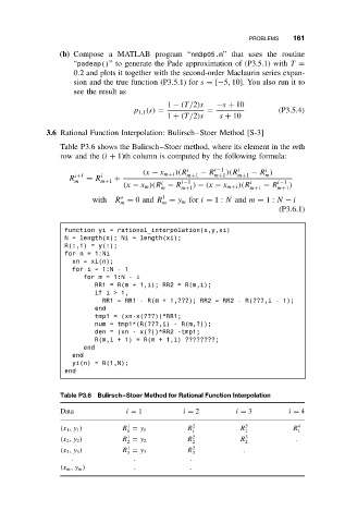
3.6 Rational Function Interpolation: Bulirsch–Stoer Method [S-3]
Table P3.6 shows the Bulirsch–Stoer method, where its element in the mth
row and the (i + 1)th column is computed by the following formula:

i−1
i
i
i
(x − x m+i )(R m+1 − R m+1 )(R m+1 − R )
m
R i+1 = R i +
m m+1 i−1 i i−1
i
(x − x m )(R − R ) − (x − x m+i )(R − R )
m m+1 m+1 m+1
1
o
with R = 0and R = y m for i = 1: N and m = 1: N − i
m
m
(P3.6.1)
function yi = rational_interpolation(x,y,xi)
N = length(x); Ni = length(xi);
R(:,1) = y(:);
for n = 1:Ni
xn = xi(n);
fori=1:N-1
form=1:N-i
RR1 = R(m + 1,i); RR2 = R(m,i);
ifi>1,
RR1 = RR1 - R(m + 1,???); RR2 = RR2 - R(???,i - 1);
end
tmp1 = (xn-x(???))*RR1;
num = tmp1*(R(???,i) - R(m,?));
den = (xn - x(?))*RR2 -tmp1;
R(m,i + 1) = R(m + 1,i) ????????;
end
end
yi(n) = R(1,N);
end
Table P3.6 Bulirsch–Stoer Method for Rational Function Interpolation
Data i = 1 i = 2 i = 3 i = 4

(x 1 ,y 1 ) 1 R 2 R 3 R 4
R = y 1
1 1 1 1
(x 2 ,y 2 ) 1 R 2 R 3 .
R = y 2
2 2 2
(x 3 ,y 3 ) 1 R 2 .
R = y 3
3 3
. . .
(x m ,y m ) . .