Page 168 - Applied Numerical Methods Using MATLAB

PROBLEMS 157
2

1
x (t )
0
: x [n]
: x (t )
–1
0 0.5 1 1.5 2 2.5 3 t = nT 3.5
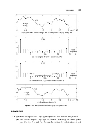
(a) A given data sequence x [n] and its interpolation x(t) by using DFS

15
|X(k)|
10

5
digital
frequency
0
0 8 16(p) 24 31 k
(b) The original DFS/DFT spectrum X(k)

15
|X′(k)|
10

5
Ws · p (2 – Ws)p digital
zero-padding(zero-out) frequency
0
0 8 16(p) 24 31 k
(c) The spectrum X′(k) of the filtered signal x′(t)
2
1 x′(t )

0 : x [n]
: x′(t )
–1
0 0.5 1 1.5 2 2.5 3 t = nT 3.5
(d) The filtered signal x′(t)
Figure 3.14 Interpolation/smoothing by using DFS/DFT.

PROBLEMS

3.1 Quadratic Interpolation: Lagrange Polynomial and Newton Polynomial
(a) The second-degree Lagrange polynomial matching the three points
(x 0 ,f 0 ), (x 1 ,f 1 ),and (x 2 ,f 2 ) can be written by substituting N = 2