Page 167 - Applied Numerical Methods Using MATLAB

156 INTERPOLATION AND CURVE FITTING

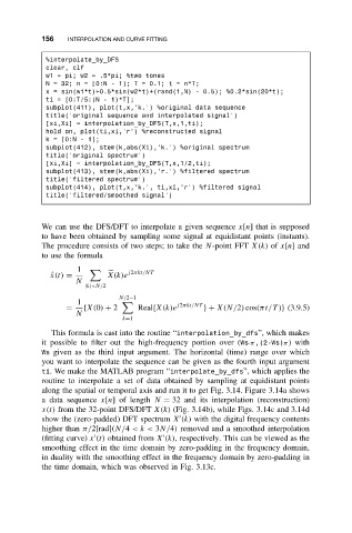
%interpolate_by_DFS
clear, clf
w1 = pi; w2 = .5*pi; %two tones
N = 32; n = [0:N - 1]; T = 0.1; t = n*T;
x = sin(w1*t)+0.5*sin(w2*t)+(rand(1,N) - 0.5); %0.2*sin(20*t);
ti = [0:T/5:(N - 1)*T];
subplot(411), plot(t,x,’k.’) %original data sequence
title(’original sequence and interpolated signal’)
[xi,Xi] = interpolation_by_DFS(T,x,1,ti);
hold on, plot(ti,xi,’r’) %reconstructed signal
k = [0:N - 1];
subplot(412), stem(k,abs(Xi),’k.’) %original spectrum
title(’original spectrum’)
[xi,Xi] = interpolation_by_DFS(T,x,1/2,ti);
subplot(413), stem(k,abs(Xi),’r.’) %filtered spectrum
title(’filtered spectrum’)
subplot(414), plot(t,x,’k.’, ti,xi,’r’) %filtered signal
title(’filtered/smoothed signal’)

We can use the DFS/DFT to interpolate a given sequence x[n] that is supposed
to have been obtained by sampling some signal at equidistant points (instants).
The procedure consists of two steps; to take the N-point FFT X(k) of x[n]and
to use the formula

1 j2πkt/NT
ˆ x(t) = X(k)e

N
|k|<N/2
N/2−1
1
= {X(0) + 2 Real{X(k)e j2πkt/NT }+ X(N/2) cos(πt/T )} (3.9.5)
N
k=1
This formula is cast into the routine “interpolation_by_dfs”, which makes
it possible to filter out the high-frequency portion over (Ws·π,(2-Ws)π) with
Ws given as the third input argument. The horizontal (time) range over which
you want to interpolate the sequence can be given as the fourth input argument
ti. We make the MATLAB program “interpolate_by_dfs”, which applies the
routine to interpolate a set of data obtained by sampling at equidistant points
along the spatial or temporal axis and run it to get Fig. 3.14. Figure 3.14a shows
a data sequence x[n]oflength N = 32 and its interpolation (reconstruction)
x(t) from the 32-point DFS/DFT X(k) (Fig. 3.14b), while Figs. 3.14c and 3.14d
show the (zero-padded) DFT spectrum X (k) with the digital frequency contents

higher than π/2[rad](N/4 <k < 3N/4) removed and a smoothed interpolation

(fitting curve) x (t) obtained from X (k), respectively. This can be viewed as the

smoothing effect in the time domain by zero-padding in the frequency domain,
in duality with the smoothing effect in the frequency domain by zero-padding in
the time domain, which was observed in Fig. 3.13c.