Page 182 - Applied Numerical Methods Using MATLAB

PROBLEMS 171
3.15 Weighted Least-Squares Curve Fitting
As in Example 3.7, we want to compare the results of applying the LS
approach and the WLS approach for finding a function that we can believe
will describe the relation between the input x and the output y as

y = ax e bx (P3.15)

where the data pair (x m , y m )’s are given as

{(1, 3.2908), (5, 3.3264), (9, 1.1640), (13, 0.3515), (17, 0.1140)}
from gauge A with error range ± 0.1
{(3, 4.7323), (7, 2.4149), (11, 0.3814), (15, −0.2396), (19, −0.2615)}
from gauge B with error range ± 0.5

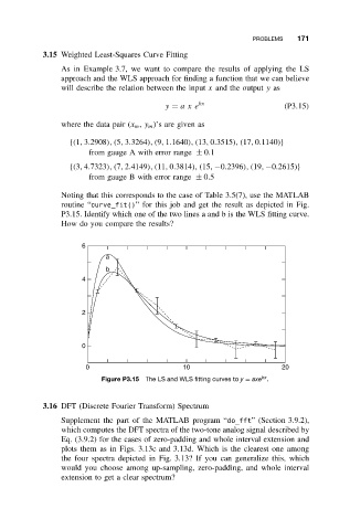
Noting that this corresponds to the case of Table 3.5(7), use the MATLAB
routine “curve_fit()” for this job and get the result as depicted in Fig.
P3.15. Identify which one of the two lines a and b is the WLS fitting curve.
How do you compare the results?

6
a
b
4

2

0

0 10 20
bx
Figure P3.15 The LS and WLS fitting curves to y = axe .

3.16 DFT (Discrete Fourier Transform) Spectrum

Supplement the part of the MATLAB program “do_fft” (Section 3.9.2),
which computes the DFT spectra of the two-tone analog signal described by
Eq. (3.9.2) for the cases of zero-padding and whole interval extension and
plots them as in Figs. 3.13c and 3.13d. Which is the clearest one among
the four spectra depicted in Fig. 3.13? If you can generalize this, which
would you choose among up-sampling, zero-padding, and whole interval
extension to get a clear spectrum?