Page 178 - Applied Numerical Methods Using MATLAB

PROBLEMS 167

%nm3p11 to plot Fig.P3.11 by curve fitting
clear
x = [1: 20]*2 - 0.1; Nx = length(x);
noise = rand(1,Nx) - 0.5; % 1xNx random noise generator
xi = [1:40]-0.5; %interpolation points
figure(1), clf
a = 0.1; b = -1; c = -50; %Table 3.5(0)
y = a*x.^2 + b*x+c+ 10*noise(1:Nx);
[th,err,yi] = curve_fit(x,y,0,2,xi); [a b c],th
[a b c],th %if you want parameters
f = inline(’th(1)*x.^2 + th(2)*x+th(3)’,’th’,’x’);
[th,err] = lsqcurvefit(f,[0 0 0],x,y), yi1 = f(th,xi);
subplot(321), plot(x,y,’*’, xi,yi,’k’, xi,yi1,’r’)
a=2;b =1;y=a./x+b+ 0.1*noise(1:Nx); %Table 3.5(1)
[th,err,yi] = curve_fit(x,y,1,0,xi); [a b],th
f = inline(’th(1)./x + th(2)’,’th’,’x’);
th0 = [0 0]; [th,err] = lsqcurvefit(f,th0,x,y), yi1 = f(th,xi);
subplot(322), plot(x,y,’*’, xi,yi,’k’, xi,yi1,’r’)
a = -20; b = -9; y = b./(x+a) + 0.4*noise(1:Nx); %Table 3.5(2)
[th,err,yi] = curve_fit(x,y,2,0,xi); [a b],th
f = inline(’th(2)./(x+th(1))’,’th’,’x’);
th0 = [0 0]; [th,err] = lsqcurvefit(f,th0,x,y), yi1 = f(th,xi);
subplot(323), plot(x,y,’*’, xi,yi,’k’, xi,yi1,’r’)
a = 2.; b = 0.95; y = a*b.^x + 0.5*noise(1:Nx); %Table 3.5(3)
[th,err,yi] = curve_fit(x,y,3,0,xi); [a b],th
f = inline(’th(1)*th(2).^x’,’th’,’x’);
th0 = [0 0]; [th,err] = lsqcurvefit(f,th0,x,y), yi1 = f(th,xi);
subplot(324), plot(x,y,’*’, xi,yi,’k’, xi,yi1,’r’)
a = 0.1; b = 1; y = b*exp(a*x) +2*noise(1:Nx); %Table 3.5(4)
[th,err,yi] = curve_fit(x,y,4,0,xi); [a b],th
f = inline(’th(2)*exp(th(1)*x)’,’th’,’x’);
th0 = [0 0]; [th,err] = lsqcurvefit(f,th0,x,y), yi1 = f(th,xi);
subplot(325), plot(x,y,’*’, xi,yi,’k’, xi,yi1,’r’)
a = 0.1; b = 1; %Table 3.5(5)
y = -b*exp(-a*x); C = -min(y)+1;y=C+y+ 0.1*noise(1:Nx);
[th,err,yi] = curve_fit(x,y,5,C,xi); [a b],th
f = inline(’1-th(2)*exp(-th(1)*x)’,’th’,’x’);
th0 = [0 0]; [th,err] = lsqcurvefit(f,th0,x,y), yi1 = f(th,xi);
subplot(326), plot(x,y,’*’, xi,yi,’k’, xi,yi1,’r’)
figure(2), clf
a = 0.5; b = 0.5; y = a*x.^b +0.2*noise(1:Nx); %Table 3.5(6a)
[th,err,yi] = curve_fit(x,y,0,2,xi); [a b],th
f = inline(’th(1)*x.^th(2)’,’th’,’x’);
th0 = [0 0]; [th,err] = lsqcurvefit(f,th0,x,y), yi1 = f(th,xi);
subplot(321), plot(x,y,’*’, xi,yi,’k’, xi,yi1,’r’)
a = 0.5; b = -0.5; %Table 3.5(6b)
y = a*x.^b + 0.05*noise(1:Nx);
[th,err,yi] = curve_fit(x,y,6,0,xi); [a b],th
f = inline(’th(1)*x.^th(2)’,’th’,’x’);
th0 = [0 0]; [th,err] = lsqcurvefit(f,th0,x,y), yi1 = f(th,xi);
subplot(322), plot(x,y,’*’, xi,yi,’k’, xi,yi1,’r’)

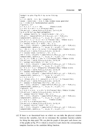
(cf) If there is no theoretical basis on which we can infer the physical relation
between the variables, how do we determine the candidate function suitable
for fitting the data pairs? We can plot the graph of data pairs and choose one
of the graphs in Fig. P3.11 which is closest to it and choose the corresponding
template function as the candidate fitting function.