Page 186 - Applied Numerical Methods Using MATLAB

PROBLEMS 175
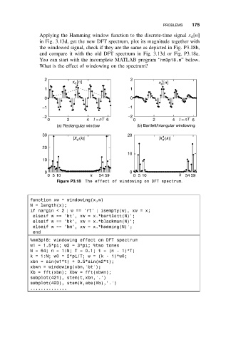
Applying the Hamming window function to the discrete-time signal x d [n]
in Fig. 3.13d, get the new DFT spectrum, plot its magnitude together with
the windowed signal, check if they are the same as depicted in Fig. P3.18b,
and compare it with the old DFT spectrum in Fig. 3.13d or Fig. P3.18a.
You can start with the incomplete MATLAB program “nm3p18.m”below.
What is the effect of windowing on the spectrum?

2 2
1
x [n] x [n]
d
d
1 1
0 0
−1 −1
−2 −2
0 2 4 t = nT 6 0 2 4 t = nT 6
(a) Rectangular window (b) Bartlett/triangular windowing
30 20
1
X (k) X (k)
d
d
20
10
10

0 0
05 10 k 54 59 05 10 k 54 59
Figure P3.18 The effect of windowing on DFT spectrum.

function xw = windowing(x,w)
N = length(x);
if nargin < 2 | w == ’rt’ | isempty(w), xw = x;
elseif w == ’bt’, xw = x.*bartlett(N)’;
elseif w == ’bk’, xw = x.*blackman(N)’;
elseif w == ’hm’, xw = x.*hamming(N)’;
end
%nm3p18: windowing effect on DFT spectrum
w1 = 1.5*pi; w2 = 3*pi; %two tones
N = 64; n = 1:N; T = 0.1;t=(n- 1)*T;
k = 1:N; w0 = 2*pi/T; w = (k - 1)*w0;
xbn = sin(w1*t) + 0.5*sin(w2*t);
xbwn = windowing(xbn,’bt’);
Xb = fft(xbn); Xbw = fft(xbwn);
subplot(421), stem(t,xbn,’.’)
subplot(423), stem(k,abs(Xb),’.’)
..............