Page 159 - Applied Numerical Methods Using MATLAB

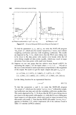
148 INTERPOLATION AND CURVE FITTING
10
10
8
8

6
6

4 linearly 4 LS linearly
interpolated
interpolated
data
data
2
2
WLS
LS
0 WLS
0
0 2 4 6 8 10 0 5 10 15 20
2 (b) Fitting to y = ax b
(a) Fitting to a polynomial y = a 2 x + a 1 x + a 0
Figure 3.11 LS curve fitting and WLS curve fitting for Example 3.7.
To find the parameters a 2 ,a 1 ,and a 0 , we write the MATLAB program
“do_wlse1.m”, which uses the routine “polyfits()” twice, once without
weighting coefficients and once with weighting coefficients. The results
are depicted in Fig. 3.11a, which shows that the WLS curve fitting tries
to be closer to the data points with smaller error bound, while the LS
curve fitting weights all data points equally, which may result in larger
deviations from data points with small error bounds.
(b) Suppose we use one gauge that has relative error bound ±40[%] for
measuring the output y for the input values x = [1, 3, 5,.. . , 19] and so
the size of error bound of each output data is proportional to the magnitude
of the output. We used it to get the input–output data pair (x m ,y m )as

{(1, 4.7334), (3, 2.1873), (5, 3.0067), (7, 1.4273), (9, 1.7787)
(11, 1.2301), (13, 1.6052), (15, 1.5353), (17, 1.3985), (19, 2.0211)}
Let the fitting function be an exponential function

y = ax b (E3.7.2)
To find the parameters a and b, we make the MATLAB program
“do_wlse2.m”, which uses the routine “curve_fit()” without the weight-
ing coefficients one time and with the weighting coefficients another time.
The results depicted in Fig. 3.11b shows that the WLS curve fitting tries to
get closer to the data points with smaller |y|, while the LS curve fitting pays
equal respect to all data points, which may result in larger deviation from
data points with small |y|. Note that the MATLAB routine “curve_fit()”
appears in Problem 3.11, which implements all of the schemes listed in
Table 3.5 with the LS/WLS solution.