Page 158 - Applied Numerical Methods Using MATLAB

CURVE FITTING 147
8 8
6 6
4 4
2 2
0 0
−2 −2
−4 −4
−4 −2 0 2 4 −4 −2 0 2 4
(a) Polynomial of degree 1 (b) Polynomial of degree 3

8 8
6 6
4 4
2 2
0 0
−2 −2
−4 −4
−4 −2 0 2 4 −4 −2 0 2 4
(c) Polynomial of degree 5 (d) Polynomial of degree 7
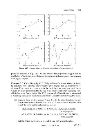
Figure 3.10 Polynomial curve fitting by the LS (Least-Squares) method.

points as depicted in Fig. 3.10. We can observe the polynomial wiggle that the
oscillation of the fitting curve between the data points becomes more pronounced
with higher degree.
Example 3.7. Curve Fitting by WLS (Weighted Least Squares). Most experimen-
tal data have some absolute and/or relative error bounds that are not uniform for
all data. If we know the error bounds for each data, we may give each data a
weight inversely proportional to the size of its error bound when extracting valu-
able information from the data. The WLS solution (3.8.7) enables us to reflect such
a weighting strategy on estimating data trends. Consider the following two cases.
(a) Suppose there are two gauges A and B with the same function, but dif-
ferent absolute error bounds ±0.2and ±1.0, respectively. We used them
to get the input-output data pair (x m ,y m )as

{(1, 0.0831), (3, 0.9290), (5, 2.4932), (7, 4.9292), (9, 7.9605)}
from gauge A
{(2, 0.9536), (4, 2.4836), (6, 3.4173), (8, 6.3903), (10, 10.2443)}
from gauge B
Let the fitting function be a second-degree polynomial function
2
y = a 2 x + a 1 x + a 0 (E3.7.1)