Page 157 - Applied Numerical Methods Using MATLAB

146 INTERPOLATION AND CURVE FITTING

function [th,err,yi] = polyfits(x,y,N,xi,r)
%x,y : the row vectors of data pairs
%N : the order of polynomial(>=0)
%r : reverse weighting factor array of the same dimension as y
M = length(x); x = x(:); y = y(:); %Make all column vectors
if nargin == 4
if length(xi) == M, r = xi; xi = x; %With input argument (x,y,N,r)
elser=1; %With input argument (x,y,N,xi)
end
elseif nargin == 3, xi = x;r=1; % With input argument (x,y,N)
end
A(:,N + 1) = ones(M,1);
for n = N:-1:1, A(:,n) = A(:,n+1).*x; end %Eq.(3.8.9)
if length(r) == M
for m = 1:M, A(m,:) = A(m,:)/r(m); y(m) = y(m)/r(m); end %Eq.(3.8.8)
end
th=(A\y)’ %Eq.(3.8.3) or (3.8.7)
ye = polyval(th,x); err = norm(y - ye)/norm(y); %estimated y values, error
yi = polyval(th,xi);

%do_polyfit
load xy1.dat
x = xy1(:,1); y = xy1(:,2);
[x,i] = sort(x); y = y(i); %sort the data for plotting
xi = min(x)+[0:100]/100*(max(x) - min(x)); %intermediate points
for i = 1:4
[th,err,yi] = polyfits(x,y,2*i - 1,xi); err %LS
subplot(220+i)
plot(x,y,’k*’,xi,yi,’b:’)
end

%xy1.dat
-3.0 -0.2774
-2.0 0.8958
-1.0 -1.5651
0.0 3.4565
1.0 3.0601
2.0 4.8568
3.0 3.8982

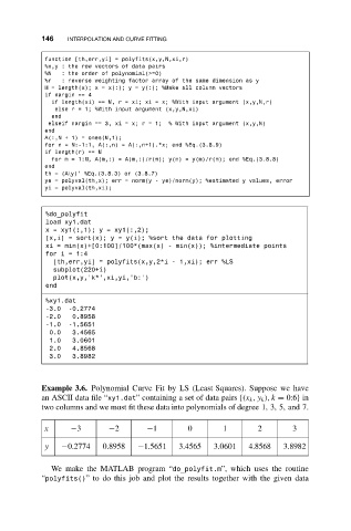
Example 3.6. Polynomial Curve Fit by LS (Least Squares). Suppose we have
an ASCII data file “xy1.dat” containing a set of data pairs {(x k ,y k ), k = 0:6} in
two columns and we must fit these data into polynomials of degree 1, 3, 5, and 7.

x −3 −2 −1 0 1 2 3

y −0.2774 0.8958 −1.5651 3.4565 3.0601 4.8568 3.8982

We make the MATLAB program “do_polyfit.m”, which uses the routine
“polyfits()” to do this job and plot the results together with the given data