Page 156 - Applied Numerical Methods Using MATLAB

CURVE FITTING 145
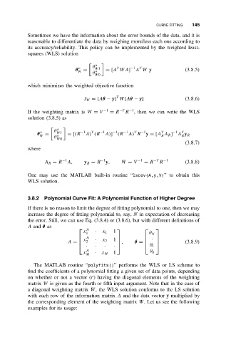
Sometimes we have the information about the error bounds of the data, and it is
reasonable to differentiate the data by weighing more/less each one according to
its accuracy/reliability. This policy can be implemented by the weighted least-
squares (WLS) solution

o
θ T −1 T
o
θ = W1 = [A WA] A W y (3.8.5)
W θ o
W0
which minimizes the weighted objective function
T
J W = [Aθ − y] W[Aθ − y] (3.8.6)
−1
If the weighting matrix is W = V −1 = R −T R , then we can write the WLS
solution (3.8.5) as

o
θ −1 T −1 −1 −1 T −1 T −1 T
o
θ W = W1 = [(R A) (R A)] (R A) R y = [A A R ] A y R
o
R
R
θ
W0
(3.8.7)
where
−1 −1 −1 −T −1
A R = R A, y R = R y, W = V = R R (3.8.8)
One may use the MATLAB built-in routine “lscov(A,y,V)” to obtain this
WLS solution.

3.8.2 Polynomial Curve Fit: A Polynomial Function of Higher Degree
If there is no reason to limit the degree of fitting polynomial to one, then we may
increase the degree of fitting polynomial to, say, N in expectation of decreasing
the error. Still, we can use Eq. (3.8.4) or (3.8.6), but with different definitions of
A and θ as
x · 1
 N   
1 x 1 θ N
 x N · x 2   · 

A = 2 1  , θ =   (3.8.9)
· · · ·
   θ 1 
x N · x M 1 θ 0
M
The MATLAB routine “polyfits()” performs the WLS or LS scheme to
find the coefficients of a polynomial fitting a given set of data points, depending
on whether or not a vector (r) having the diagonal elements of the weighting
matrix W is given as the fourth or fifth input argument. Note that in the case of
a diagonal weighting matrix W, the WLS solution conforms to the LS solution
with each row of the information matrix A and the data vector y multiplied by
the corresponding element of the weighting matrix W. Let us see the following
examples for its usage: